Getting started with hillmaker#
In this tutorial we’ll focus on basic use of hillmaker for analyzing arrivals, departures, and occupancy by time of day and day of week for a typical discrete entity flow system. A few examples of such systems include:
patients arriving, undergoing some sort of care process and departing some healthcare system (e.g. emergency department, surgical recovery, nursing unit, outpatient clinic, and many more)
customers renting, using, and returning bikes in a bike share system,
users of licensed software checking out, using, checking back in a software license,
products undergoing some sort of manufacturing or assembly process - occupancy is WIP,
patrons arriving, dining and leaving a restaurant,
travelers renting, residing in, and checking out of a hotel,
flights taking off and arriving at their destination,
…
Basically, any sort of discrete stock and flow system for which you are interested in time of day and day of week specific statistical summaries of occupancy, arrivals and departures, and have raw data on the arrival and departure times, is fair game for hillmaker.
Installation#
You can use pip to install hillmaker into the Python virtual environment of your choice.
pip install hillmaker
You should also be able to install hillmaker from conda-forge shortly into a virtual environment.
conda config --add channels conda-forge
conda config --set channel_priority strict
conda install hillmaker
If you want to get the latest update which is not yet on PyPI or conda-forge, you can install from the GitHub repo’s develop branch:
pip install git+https://github.com/misken/hillmaker@develop
Getting this notebook and sample data#
If you want to get a copy of this notebook to try out the examples yourself, the easiest way to get it is to go to the companion hillmaker-examples repo and either clone it or download it as a zip file. You’ll find several notebooks in there including this getting_started.ipynb file. A few sample data files are included in the data folder - including the ssu_2024.csv file used for this demo.
After opening any of the notebooks, make sure you set your Jupyter kernel to whichever conda virtual environment contains the installed version of hillmaker.
Ways of using hillmaker#
There are currently three ways of using hillmaker.
Command line interface (CLI)
Calling a single Python function
An object oriented API in Python
The plan is to add a fourth option:
Through a GUI interface (not implemented yet)
Depending on your level of comfort with Python, you can choose the method that works best for you. This Getting Started tutorial will demo all three ways of using hillmaker and subsequent tutorials will go into more detail. There are numerous input parameters that can be used to customize the behavior of hillmaker and we’ll only touch on a few in this tutorial.
Module imports#
To run hillmaker we only need to import a few modules. Often we will be using pandas as part of our analysis and we’ll import that as well.
from pathlib import Path
import pandas as pd
import hillmaker as hm
A prototypical example - occupancy analysis of a hospital Short Stay Unit#
Patients flow through a short stay unit (SSU) for a variety of procedures, tests or therapies. Let’s assume patients can be classified into one of five categories of patient types: ART (arterialgram), CAT (post cardiac-cath), MYE (myelogram), IVT (IV therapy), and OTH (other). We are interested in occupancy statistics by time of day and day of week to support things like staff scheduling and capacity planning.
From one of our hospital information systems we were able to get raw data about the entry and exit times of each patient and exported the data to a csv file. We call each row of such data a stop (as in, the patient stopped here for a while). Let’s take a peek at the data by first reading the csv file into a pandas DataFrame.
ssu_stopdata = 'https://raw.githubusercontent.com/misken/hillmaker-examples/main/data/ssu_2024.csv'
# ssu_stopdata = './data/ssu_2024.csv'
stops_df = pd.read_csv(ssu_stopdata, parse_dates=['InRoomTS','OutRoomTS'])
stops_df.info()
<class 'pandas.core.frame.DataFrame'>
RangeIndex: 59877 entries, 0 to 59876
Data columns (total 5 columns):
 #   Column     Non-Null Count  Dtype
---  ------     --------------  -----
 0   PatID      59877 non-null  int64
 1   InRoomTS   59877 non-null  datetime64[ns]
 2   OutRoomTS  59877 non-null  datetime64[ns]
 3   PatType    59877 non-null  object
 4   LOS_hours  59877 non-null  float64
dtypes: datetime64[ns](2), float64(1), int64(1), object(1)
memory usage: 2.3+ MB
stops_df.head()
| PatID | InRoomTS | OutRoomTS | PatType | LOS_hours | |
|---|---|---|---|---|---|
| 0 | 1 | 2024-01-01 07:44:00 | 2024-01-01 09:20:00 | IVT | 1.600000 |
| 1 | 2 | 2024-01-01 08:28:00 | 2024-01-01 11:13:00 | IVT | 2.750000 |
| 2 | 3 | 2024-01-01 11:44:00 | 2024-01-01 12:48:00 | MYE | 1.066667 |
| 3 | 4 | 2024-01-01 11:51:00 | 2024-01-01 21:10:00 | CAT | 9.316667 |
| 4 | 5 | 2024-01-01 12:10:00 | 2024-01-01 12:57:00 | IVT | 0.783333 |
Before running hillmaker, we need to know the timeframe for which we have data.
stops_df['InRoomTS'].min()
Timestamp('2024-01-01 07:44:00')
stops_df['InRoomTS'].max()
Timestamp('2024-09-30 22:45:00')
Looks like we have data from Jan through Sept of 2024. Since patients usually stay for less than 24 hours in an SSU, we’ll do our occupancy analysis starting on January 2, 2024 (since the 1st is a holiday) and ending on September 30, 2024. Later in the tutorial we’ll discuss the important issues of choosing an appropriate analysis timeframe and horizon effects.
As part of an operational analysis we would like to compute a number of relevant statistics, such as:
mean and 95th percentile of overall SSU occupancy by hour of day and day of week,
similar hourly statistics for patient arrivals and departures,
all of the above but by patient type as well.
In addition to tabular summaries, let’s make some plots showing the mean and 95th percentile of occupancy by time of day and day of week.
Running hillmaker via the command line interface (CLI)#
To run hillmaker from the command line, make sure that you are using whatever virtual environment within which hillmaker is installed. Let’s see the help for hillmaker’s CLI:
> hillmaker -h
usage: hillmaker [--scenario_name SCENARIO_NAME] [--data DATA]
                 [--in_field IN_FIELD] [--out_field OUT_FIELD]
                 [--start_analysis_dt START_ANALYSIS_DT]
                 [--end_analysis_dt END_ANALYSIS_DT] [--config CONFIG]
                 [--cat_field CAT_FIELD] [--bin_size_minutes BIN_SIZE_MINUTES]
                 [--cats_to_exclude [CATS_TO_EXCLUDE ...]]
                 [--occ_weight_field OCC_WEIGHT_FIELD]
                 [--percentiles [PERCENTILES ...]] [--los_units LOS_UNITS]
                 [--csv_export_path CSV_EXPORT_PATH] [--no_dow_plots]
                 [--no_week_plots] [--plot_export_path PLOT_EXPORT_PATH]
                 [--plot_style PLOT_STYLE] [--figsize FIGSIZE FIGSIZE]
                 [--bar_color_mean BAR_COLOR_MEAN] [--alpha ALPHA]
                 [--plot_percentiles PLOT_PERCENTILES [PLOT_PERCENTILES ...]]
                 [--pctile_color PCTILE_COLOR [PCTILE_COLOR ...]]
                 [--pctile_linestyle PCTILE_LINESTYLE [PCTILE_LINESTYLE ...]]
                 [--pctile_linewidth [PCTILE_LINEWIDTH ...]] [--cap CAP]
                 [--cap_color CAP_COLOR] [--xlabel XLABEL] [--ylabel YLABEL]
                 [--main_title MAIN_TITLE] [--subtitle SUBTITLE]
                 [--first_dow FIRST_DOW] [--edge_bins EDGE_BINS]
                 [--highres_bin_size_minutes HIGHRES_BIN_SIZE_MINUTES]
                 [--keep_highres_bydatetime] [--verbosity VERBOSITY] [-h]

Occupancy analysis by time of day and day of week

Required arguments (either on command line or via config file):
  --scenario_name SCENARIO_NAME
                        Used in output filenames
  --data DATA           Path to csv file containing the stop data to be
                        processed
  --in_field IN_FIELD   Column name corresponding to the arrival times
  --out_field OUT_FIELD
                        Column name corresponding to the departure times
  --start_analysis_dt START_ANALYSIS_DT
                        Starting datetime for the analysis (use yyyy-mm-dd
                        format)
  --end_analysis_dt END_ANALYSIS_DT
                        Ending datetime for the analysis (use yyyy-mm-dd
                        format)

Optional arguments:
  --config CONFIG       Configuration file (TOML format) containing input
                        parameter arguments and values. Input parameters set
                        via a config file will override parameters values
                        passed via the command line.
  --cat_field CAT_FIELD
                        Column name corresponding to the categories. If None,
                        then only overall occupancy is analyzed.
  --bin_size_minutes BIN_SIZE_MINUTES
                        Number of minutes in each time bin of the day
                        (default=60) for aggregate statistics and plots.
  --cats_to_exclude [CATS_TO_EXCLUDE ...]
                        Category values to exclude from the analysis.
  --occ_weight_field OCC_WEIGHT_FIELD
                        Column name corresponding to occupancy weights. If
                        None, then weight of 1.0 is used. Default is None.
  --percentiles [PERCENTILES ...]
                        Which percentiles to compute
  --los_units LOS_UNITS
                        The time units for length of stay analysis. See https:
                        //pandas.pydata.org/docs/reference/api/pandas.Timedelt
                        a.html for allowable values (smallest value allowed is
                        'seconds', largest is 'days'. The default is 'hours'.
  --csv_export_path CSV_EXPORT_PATH
                        Destination path for exported csv files, default is
                        current directory.
  --no_dow_plots        If set, no day of week plots are created.
  --no_week_plots       If set, no weekly plots are created.
  --plot_export_path PLOT_EXPORT_PATH
                        Destination path for exported plots, default is
                        current directory.
  --plot_style PLOT_STYLE
                        Matplotlib style name.
  --figsize FIGSIZE FIGSIZE
                        Figure size
  --bar_color_mean BAR_COLOR_MEAN
                        Matplotlib color name for the bars representing mean
                        values.
  --alpha ALPHA         Transparency for bars, default=0.5.
  --plot_percentiles PLOT_PERCENTILES [PLOT_PERCENTILES ...]
                        Which percentiles to plot
  --pctile_color PCTILE_COLOR [PCTILE_COLOR ...]
                        Line color for each percentile series plotted. Order
                        should match order of percentiles list.
  --pctile_linestyle PCTILE_LINESTYLE [PCTILE_LINESTYLE ...]
                        Line style for each percentile series plotted.
  --pctile_linewidth [PCTILE_LINEWIDTH ...]
                        Line width for each percentile series plotted.
  --cap CAP             Capacity level line to include in occupancy plots
  --cap_color CAP_COLOR
                        Matplotlib color code.
  --xlabel XLABEL       x-axis label for plots.
  --ylabel YLABEL       y-axis label for plots.
  --main_title MAIN_TITLE
                        Main title for plot. Default = '{Occupancy, Arrivals,
                        Departures} by time of day and day of week'
  --subtitle SUBTITLE   Subtitle for plot. Default = 'Scenario:
                        {scenario_name}'
  --first_dow FIRST_DOW
                        Controls which day of week appears first in plot. One
                        of 'mon', 'tue', 'wed', 'thu', 'fri', 'sat, 'sun'
  -h, --help

Advanced optional arguments:
  --edge_bins EDGE_BINS
                        Occupancy contribution method for arrival and
                        departure bins. 1=fractional, 2=entire bin
  --highres_bin_size_minutes HIGHRES_BIN_SIZE_MINUTES
                        Number of minutes in each time bin of the day used for
                        initial computation of the number of arrivals,
                        departures, and the occupancy level. This value should
                        be <= `bin_size_minutes`. The shorter the duration of
                        stays, the smaller the resolution should be if using
                        edge_bins=2. See docs for more details.
  --keep_highres_bydatetime
                        Save the high resolution bydatetime dataframe in hills
                        attribute.
  --verbosity VERBOSITY
                        Used to set level in loggers. 0=logging.WARNING,
                        1=logging.INFO (default), 2=logging.DEBUG
There are several required arguments:
SCENARIO_NAME - a scenario name,
DATA - the path to the csv file containing the stop data,
IN_FIELD, OUT_FIELD - the field names containing the arrival times and the departure times,
START_ANALYSIS_DT, END_ANALYSIS_DT - starting and ending dates for the analysis.
There are also numerous optional arguments controlling how hillmaker works and which outputs are created.
Let’s run hillmaker by specifying the required arguments as well as an output path for plots and csv files. The stop data file, ssu_2024.csv is in the data folder. We’ll output plots and csv summary files to the output folder. Typically, we would also specify a category field - in this case it would be PatType. We’ll use 60 minutes for the time bin size.
By default, hillmaker prints out several informational messages. You can suppress these with --verbosity 0. You can get even more detailed status messages (useful for debugging) by using --verbosity 2.
> hillmaker --scenario cli_demo_ssu_60 --data ./data/ssu_2024.csv \
--in_field InRoomTS --out_field OutRoomTS --cat_field PatType --bin_size_minutes 60 \
--start_analysis_dt 2024-01-02 --end_analysis_dt 2024-09-30 --csv_export_path output --plot_export_path output --ylabel Patients
2024-01-16 09:47:56,728 - hillmaker.hills - INFO - Starting scenario cli_demo_ssu_60
2024-01-16 09:48:05,516 - hillmaker.summarize - INFO - Created nonstationary summaries - ['PatType']
2024-01-16 09:48:06,635 - hillmaker.summarize - INFO - Created nonstationary summaries - []
2024-01-16 09:48:06,668 - hillmaker.summarize - INFO - Created stationary summaries - ['PatType']
2024-01-16 09:48:06,679 - hillmaker.summarize - INFO - Created stationary summaries - []
2024-01-16 09:48:08,173 - hillmaker.hills - INFO - bydatetime and summaries by datetime created (seconds): 11.3838
2024-01-16 09:48:08,419 - hillmaker.hills - INFO - By datetime exported to csv in output (seconds): 0.2408
2024-01-16 09:48:08,492 - hillmaker.hills - INFO - Summaries exported to csv in output (seconds): 0.0733
2024-01-16 09:48:10,683 - hillmaker.plotting - INFO - Full week plots created (seconds): 2.1840
2024-01-16 09:48:19,486 - hillmaker.plotting - INFO - Individual day of week plots created (seconds): 8.8003
2024-01-16 09:48:19,486 - hillmaker.hills - INFO - Total time (seconds): 22.6828
CSV file outputs#
When you use the CLI, CSV versions of the output tables are exported to CSV_EXPORT_PATH.
There are four groups of files, each beginning with the scenario name 'cli_demo_ssu_60'.
occupancy,arrivals,departures- summary statistics for occupancy, arrivals and departuresbydatetime- number of arrivals, departures and occupancy level by datetime bin over the analysis range (e.g. individual hours on each date)
Usually it’s the occupancy summaries that we are most interested in. From each occupancy related filename, we can infer the grouping levels used for the summary statistics.
<scenario name>_occupancy_dow_binofday.csv#
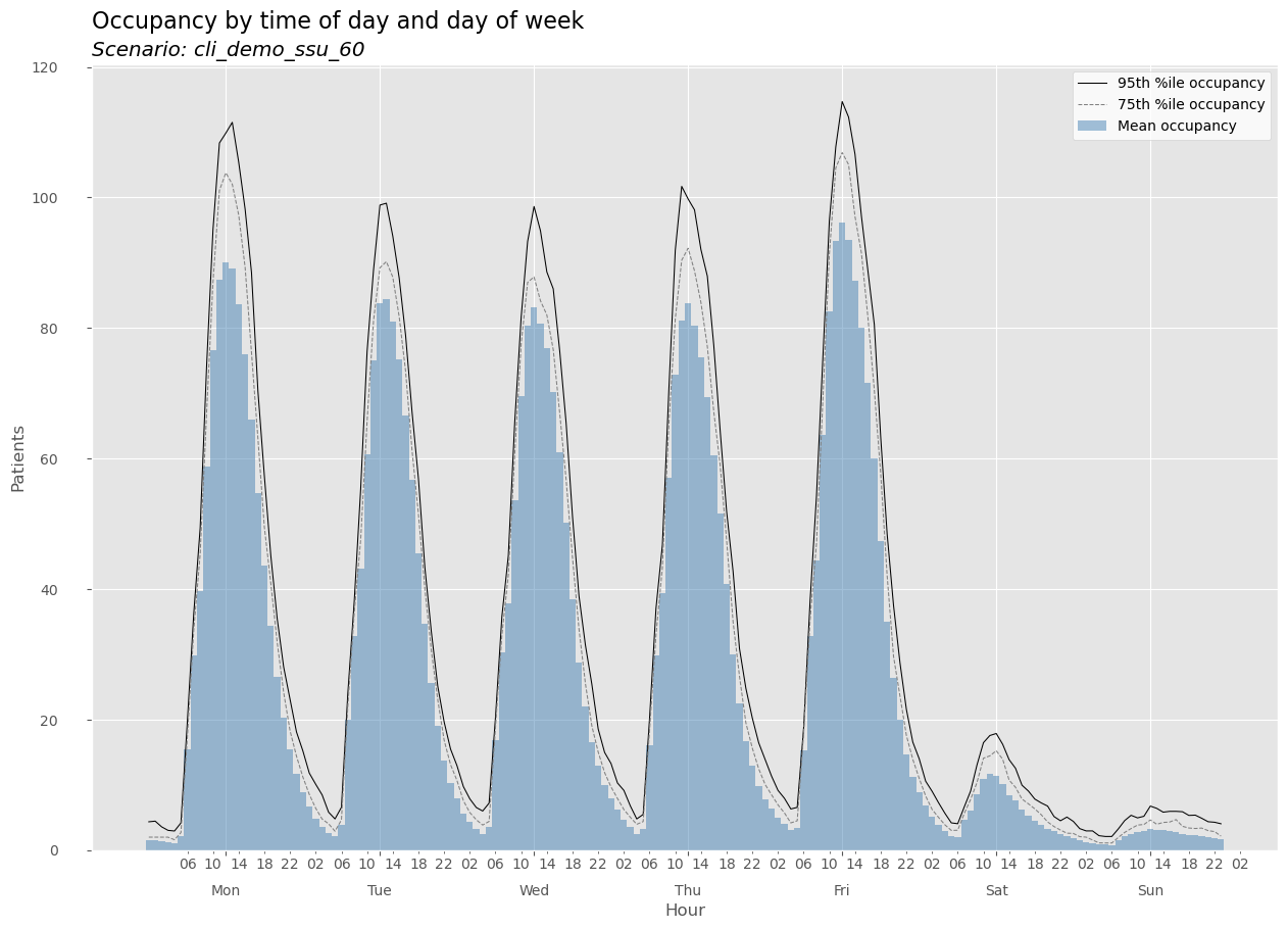
This is probably the most used summary as it gives us overall occupancy statistics by time bin of day (in this case, hourly) and day of week. We can read it into a pandas DataFrame and take a look. Since we used hourly time bins, there will be 168 rows in the summary. Numerous summary statistics are computed for each hour of the week.
occ_dow_binofday_df = pd.read_csv('output/cli_demo_ssu_60_occupancy_dow_binofday.csv')
occ_dow_binofday_df.head(30)
| day_of_week | dow_name | bin_of_day | bin_of_day_str | count | mean | min | max | stdev | sem | var | cv | skew | kurt | p25 | p50 | p75 | p95 | p99 | |
|---|---|---|---|---|---|---|---|---|---|---|---|---|---|---|---|---|---|---|---|
| 0 | 0 | Mon | 0 | 00:00 | 39.0 | 1.561966 | 0.000000 | 4.666667 | 1.337969 | 0.214246 | 1.790160 | 0.856593 | 0.863336 | -0.009379 | 0.533333 | 1.000000 | 2.000000 | 4.353333 | 4.616000 |
| 1 | 0 | Mon | 1 | 01:00 | 39.0 | 1.530342 | 0.000000 | 5.000000 | 1.314454 | 0.210481 | 1.727791 | 0.858929 | 1.123432 | 0.861793 | 0.783333 | 1.000000 | 2.000000 | 4.450000 | 4.905000 |
| 2 | 0 | Mon | 2 | 02:00 | 39.0 | 1.364103 | 0.000000 | 4.950000 | 1.194374 | 0.191253 | 1.426528 | 0.875575 | 1.089267 | 1.091913 | 0.950000 | 1.000000 | 2.000000 | 3.578333 | 4.582667 |
| 3 | 0 | Mon | 3 | 03:00 | 39.0 | 1.232479 | 0.000000 | 4.400000 | 1.058411 | 0.169481 | 1.120233 | 0.858766 | 0.875510 | 0.792365 | 0.350000 | 1.000000 | 1.991667 | 3.040000 | 4.020000 |
| 4 | 0 | Mon | 4 | 04:00 | 39.0 | 1.076068 | 0.000000 | 3.900000 | 0.971568 | 0.155575 | 0.943944 | 0.902887 | 0.893486 | 0.663040 | 0.000000 | 1.000000 | 1.600000 | 2.940000 | 3.558000 |
| 5 | 0 | Mon | 5 | 05:00 | 39.0 | 2.229915 | 0.083333 | 4.700000 | 1.138399 | 0.182290 | 1.295953 | 0.510513 | 0.442054 | -0.335741 | 1.508333 | 2.000000 | 2.691667 | 4.178333 | 4.598667 |
| 6 | 0 | Mon | 6 | 06:00 | 39.0 | 15.443162 | 0.333333 | 21.483333 | 3.931664 | 0.629570 | 15.457978 | 0.254589 | -2.423603 | 7.778248 | 14.616667 | 16.083333 | 17.241667 | 19.630000 | 21.166667 |
| 7 | 0 | Mon | 7 | 07:00 | 39.0 | 29.869658 | 1.533333 | 38.966667 | 7.498266 | 1.200683 | 56.223989 | 0.251033 | -2.669468 | 8.294117 | 28.625000 | 31.433333 | 33.708333 | 36.283333 | 38.346000 |
| 8 | 0 | Mon | 8 | 08:00 | 39.0 | 39.738889 | 1.683333 | 56.650000 | 10.724470 | 1.717290 | 115.014259 | 0.269873 | -2.304590 | 6.600737 | 36.925000 | 42.650000 | 45.366667 | 49.335000 | 54.218000 |
| 9 | 0 | Mon | 9 | 09:00 | 39.0 | 58.750000 | 1.483333 | 79.116667 | 15.509799 | 2.483556 | 240.553874 | 0.263997 | -2.538838 | 7.735264 | 57.241667 | 61.283333 | 66.858333 | 74.036667 | 77.311667 |
| 10 | 0 | Mon | 10 | 10:00 | 39.0 | 76.657265 | 2.933333 | 96.083333 | 19.943244 | 3.193475 | 397.732994 | 0.260161 | -2.639291 | 8.119880 | 72.983333 | 80.550000 | 87.066667 | 95.083333 | 95.874333 |
| 11 | 0 | Mon | 11 | 11:00 | 39.0 | 87.416239 | 1.733333 | 110.083333 | 22.724800 | 3.638880 | 516.416557 | 0.259961 | -2.657434 | 8.241843 | 81.450000 | 92.700000 | 101.083333 | 108.351667 | 109.659000 |
| 12 | 0 | Mon | 12 | 12:00 | 39.0 | 90.031197 | 1.233333 | 112.683333 | 23.185833 | 3.712705 | 537.582854 | 0.257531 | -2.770866 | 8.875578 | 85.091667 | 95.283333 | 103.783333 | 109.875000 | 112.613667 |
| 13 | 0 | Mon | 13 | 13:00 | 39.0 | 89.194872 | 1.716667 | 114.500000 | 23.579497 | 3.775741 | 555.992663 | 0.264359 | -2.536764 | 7.819967 | 81.883333 | 94.900000 | 102.033333 | 111.513333 | 114.265667 |
| 14 | 0 | Mon | 14 | 14:00 | 39.0 | 83.608120 | 1.000000 | 109.900000 | 22.223400 | 3.558592 | 493.879501 | 0.265804 | -2.464217 | 7.522566 | 78.233333 | 85.833333 | 97.308333 | 105.406667 | 108.329333 |
| 15 | 0 | Mon | 15 | 15:00 | 39.0 | 75.979060 | 0.700000 | 100.933333 | 20.640815 | 3.305176 | 426.043227 | 0.271665 | -2.237832 | 6.670489 | 69.666667 | 77.233333 | 89.283333 | 98.213333 | 100.401333 |
| 16 | 0 | Mon | 16 | 16:00 | 39.0 | 65.939744 | 0.000000 | 89.616667 | 18.346099 | 2.937727 | 336.579336 | 0.278225 | -2.003630 | 5.710318 | 60.600000 | 67.816667 | 76.200000 | 88.478333 | 89.395000 |
| 17 | 0 | Mon | 17 | 17:00 | 39.0 | 54.656838 | 0.000000 | 74.916667 | 14.673648 | 2.349664 | 215.315932 | 0.268469 | -2.208259 | 6.392677 | 52.000000 | 57.250000 | 63.083333 | 70.353333 | 74.448000 |
| 18 | 0 | Mon | 18 | 18:00 | 39.0 | 43.552137 | 0.000000 | 59.950000 | 11.772127 | 1.885049 | 138.582970 | 0.270300 | -2.067508 | 5.864829 | 40.391667 | 46.016667 | 49.500000 | 57.355000 | 59.608000 |
| 19 | 0 | Mon | 19 | 19:00 | 39.0 | 34.383761 | 0.000000 | 54.766667 | 10.059813 | 1.610859 | 101.199832 | 0.292575 | -1.417011 | 3.653496 | 29.341667 | 36.566667 | 40.950000 | 45.165000 | 51.283333 |
| 20 | 0 | Mon | 20 | 20:00 | 39.0 | 26.618803 | 0.000000 | 43.683333 | 8.012713 | 1.283061 | 64.203570 | 0.301017 | -1.041871 | 2.649560 | 22.608333 | 28.000000 | 31.841667 | 35.450000 | 41.010667 |
| 21 | 0 | Mon | 21 | 21:00 | 39.0 | 20.254274 | 0.233333 | 32.533333 | 6.076123 | 0.972958 | 36.919265 | 0.299992 | -0.874277 | 2.225625 | 17.108333 | 20.183333 | 24.166667 | 28.080000 | 31.399667 |
| 22 | 0 | Mon | 22 | 22:00 | 39.0 | 15.472650 | 1.000000 | 24.483333 | 4.632457 | 0.741787 | 21.459656 | 0.299396 | -0.580108 | 1.556255 | 12.958333 | 15.766667 | 18.283333 | 23.061667 | 24.439000 |
| 23 | 0 | Mon | 23 | 23:00 | 39.0 | 11.723932 | 0.950000 | 19.833333 | 4.014841 | 0.642889 | 16.118944 | 0.342448 | -0.146289 | 0.260521 | 9.275000 | 11.483333 | 14.408333 | 18.121667 | 19.314000 |
| 24 | 1 | Tue | 0 | 00:00 | 39.0 | 8.926496 | 1.000000 | 15.633333 | 3.631447 | 0.581497 | 13.187408 | 0.406817 | -0.088015 | -0.365883 | 6.458333 | 8.883333 | 11.216667 | 15.211667 | 15.570000 |
| 25 | 1 | Tue | 1 | 01:00 | 39.0 | 6.629915 | 0.883333 | 13.816667 | 3.112203 | 0.498351 | 9.685807 | 0.469418 | 0.441786 | -0.255520 | 4.025000 | 6.983333 | 8.550000 | 11.815000 | 13.677333 |
| 26 | 1 | Tue | 2 | 02:00 | 39.0 | 4.836325 | 0.000000 | 12.133333 | 2.821619 | 0.451821 | 7.961533 | 0.583422 | 0.722422 | 0.367211 | 3.000000 | 4.100000 | 6.425000 | 10.100000 | 11.702667 |
| 27 | 1 | Tue | 3 | 03:00 | 39.0 | 3.550000 | 0.000000 | 9.016667 | 2.295088 | 0.367508 | 5.267427 | 0.646504 | 0.842881 | 0.299023 | 2.000000 | 3.116667 | 4.766667 | 8.466667 | 8.978667 |
| 28 | 1 | Tue | 4 | 04:00 | 39.0 | 2.684188 | 0.000000 | 7.000000 | 1.849585 | 0.296171 | 3.420964 | 0.689067 | 0.446491 | -0.723028 | 1.066667 | 2.533333 | 4.050000 | 5.823333 | 6.575667 |
| 29 | 1 | Tue | 5 | 05:00 | 39.0 | 2.081624 | 0.000000 | 7.316667 | 1.668520 | 0.267177 | 2.783959 | 0.801547 | 0.893497 | 1.093824 | 0.766667 | 2.000000 | 2.908333 | 4.790000 | 6.436333 |
From the count field we can see that there were 39 Mondays in the analysis date range. It is this DataFrame that used to create the weekly and day of week plots.
Plots are created in PNG format and exported to PLOT_EXPORT_PATH.
[fname.name for fname in Path('output/').glob('cli_demo_ssu_60*occupancy*.png')]
['cli_demo_ssu_60_occupancy_week.png',
 'cli_demo_ssu_60_occupancy_thu.png',
 'cli_demo_ssu_60_occupancy_mon.png',
 'cli_demo_ssu_60_occupancy_tue.png',
 'cli_demo_ssu_60_occupancy_fri.png',
 'cli_demo_ssu_60_occupancy_sun.png',
 'cli_demo_ssu_60_occupancy_sat.png',
 'cli_demo_ssu_60_occupancy_wed.png']
from IPython.display import Image
Image('output/cli_demo_ssu_60_occupancy_week.png')
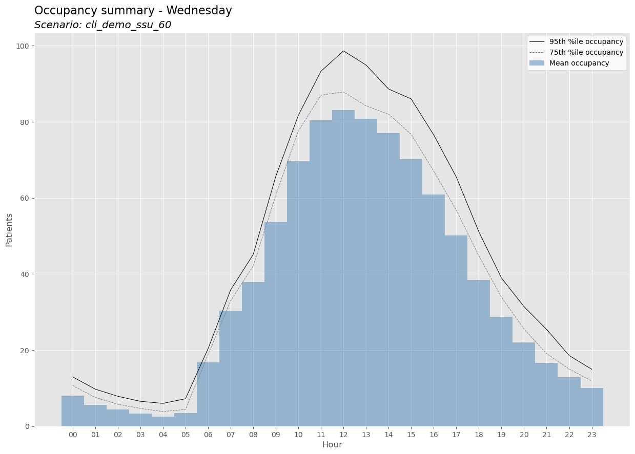
There are also day of week specific plots.
Image('output/cli_demo_ssu_60_occupancy_wed.png')
<scenario name>_PatType_dow_binofday.csv#
This is the most detailed summary as it is grouped by category (patient type in this example), day of week and hour of day. This DataFrame is useful for seeing how individual patient types contribute to overall occupancy in the SSU.
occ_PatType_dow_binofday_df = pd.read_csv('output/cli_demo_ssu_60_occupancy_PatType_dow_binofday.csv')
occ_PatType_dow_binofday_df.iloc[50:75]
| PatType | day_of_week | dow_name | bin_of_day | bin_of_day_str | count | mean | min | max | stdev | sem | var | cv | skew | kurt | p25 | p50 | p75 | p95 | p99 | |
|---|---|---|---|---|---|---|---|---|---|---|---|---|---|---|---|---|---|---|---|---|
| 50 | ART | 2 | Wed | 2 | 02:00 | 39.0 | 0.000000 | 0.000000 | 0.000000 | 0.000000 | 0.000000 | 0.000000 | 0.000000 | 0.000000 | 0.000000 | 0.000000 | 0.000000 | 0.000000 | 0.000000 | 0.000000 |
| 51 | ART | 2 | Wed | 3 | 03:00 | 39.0 | 0.000000 | 0.000000 | 0.000000 | 0.000000 | 0.000000 | 0.000000 | 0.000000 | 0.000000 | 0.000000 | 0.000000 | 0.000000 | 0.000000 | 0.000000 | 0.000000 |
| 52 | ART | 2 | Wed | 4 | 04:00 | 39.0 | 0.000000 | 0.000000 | 0.000000 | 0.000000 | 0.000000 | 0.000000 | 0.000000 | 0.000000 | 0.000000 | 0.000000 | 0.000000 | 0.000000 | 0.000000 | 0.000000 |
| 53 | ART | 2 | Wed | 5 | 05:00 | 39.0 | 0.358120 | 0.000000 | 1.333333 | 0.377373 | 0.060428 | 0.142410 | 1.053762 | 1.100851 | 0.604813 | 0.008333 | 0.250000 | 0.575000 | 1.180000 | 1.320667 |
| 54 | ART | 2 | Wed | 6 | 06:00 | 39.0 | 3.672222 | 1.683333 | 5.716667 | 1.031559 | 0.165182 | 1.064113 | 0.280909 | 0.059364 | -0.694543 | 3.008333 | 3.516667 | 4.408333 | 5.183333 | 5.628000 |
| 55 | ART | 2 | Wed | 7 | 07:00 | 39.0 | 7.820940 | 4.966667 | 10.633333 | 1.385444 | 0.221849 | 1.919455 | 0.177145 | 0.012103 | -0.394016 | 6.900000 | 7.600000 | 8.875000 | 9.788333 | 10.614333 |
| 56 | ART | 2 | Wed | 8 | 08:00 | 39.0 | 10.516239 | 6.466667 | 15.383333 | 2.184222 | 0.349755 | 4.770826 | 0.207700 | 0.452734 | -0.204397 | 9.291667 | 10.083333 | 11.633333 | 14.235000 | 15.237667 |
| 57 | ART | 2 | Wed | 9 | 09:00 | 39.0 | 12.370940 | 6.833333 | 20.316667 | 2.871884 | 0.459869 | 8.247715 | 0.232148 | 0.561270 | 0.441556 | 10.591667 | 12.000000 | 14.108333 | 17.330000 | 19.341333 |
| 58 | ART | 2 | Wed | 10 | 10:00 | 39.0 | 13.094017 | 8.250000 | 22.400000 | 2.954995 | 0.473178 | 8.731995 | 0.225675 | 0.862908 | 1.336721 | 11.350000 | 12.716667 | 15.008333 | 17.261667 | 21.114333 |
| 59 | ART | 2 | Wed | 11 | 11:00 | 39.0 | 13.336752 | 7.683333 | 21.333333 | 2.775359 | 0.444413 | 7.702620 | 0.208099 | 0.999808 | 1.666926 | 11.916667 | 12.766667 | 14.266667 | 19.376667 | 20.909000 |
| 60 | ART | 2 | Wed | 12 | 12:00 | 39.0 | 13.040598 | 8.316667 | 19.433333 | 2.560224 | 0.409964 | 6.554748 | 0.196327 | 0.492908 | 0.419179 | 11.383333 | 12.733333 | 14.683333 | 17.041667 | 19.408000 |
| 61 | ART | 2 | Wed | 13 | 13:00 | 39.0 | 11.941026 | 8.716667 | 17.983333 | 2.236499 | 0.358126 | 5.001928 | 0.187295 | 0.692769 | 0.055469 | 10.158333 | 11.633333 | 13.158333 | 15.430000 | 17.400667 |
| 62 | ART | 2 | Wed | 14 | 14:00 | 39.0 | 9.993162 | 4.300000 | 16.133333 | 2.498238 | 0.400038 | 6.241195 | 0.249995 | -0.040163 | 0.074037 | 8.591667 | 9.883333 | 11.683333 | 13.605000 | 15.246667 |
| 63 | ART | 2 | Wed | 15 | 15:00 | 39.0 | 7.287607 | 2.000000 | 13.616667 | 2.672925 | 0.428011 | 7.144528 | 0.366777 | 0.182371 | 0.306827 | 5.808333 | 7.000000 | 9.008333 | 12.061667 | 13.464667 |
| 64 | ART | 2 | Wed | 16 | 16:00 | 39.0 | 5.062821 | 1.000000 | 10.316667 | 2.303012 | 0.368777 | 5.303866 | 0.454887 | 0.262786 | -0.271186 | 3.258333 | 5.000000 | 6.708333 | 8.330000 | 10.291333 |
| 65 | ART | 2 | Wed | 17 | 17:00 | 39.0 | 3.279915 | 0.350000 | 7.950000 | 1.934457 | 0.309761 | 3.742123 | 0.589789 | 0.603736 | -0.200242 | 1.975000 | 3.000000 | 4.616667 | 6.926667 | 7.766333 |
| 66 | ART | 2 | Wed | 18 | 18:00 | 39.0 | 1.961538 | 0.000000 | 5.833333 | 1.525045 | 0.244203 | 2.325762 | 0.777474 | 0.713760 | -0.158408 | 0.875000 | 1.833333 | 2.975000 | 4.651667 | 5.561000 |
| 67 | ART | 2 | Wed | 19 | 19:00 | 39.0 | 1.068803 | 0.000000 | 4.000000 | 1.084218 | 0.173614 | 1.175529 | 1.014422 | 0.929103 | 0.299327 | 0.000000 | 1.000000 | 1.641667 | 3.270000 | 3.734000 |
| 68 | ART | 2 | Wed | 20 | 20:00 | 39.0 | 0.683333 | 0.000000 | 3.716667 | 0.950854 | 0.152258 | 0.904123 | 1.391493 | 1.525316 | 1.818134 | 0.000000 | 0.033333 | 1.000000 | 2.433333 | 3.400000 |
| 69 | ART | 2 | Wed | 21 | 21:00 | 39.0 | 0.367949 | 0.000000 | 2.216667 | 0.681892 | 0.109190 | 0.464976 | 1.853225 | 1.752237 | 1.752261 | 0.000000 | 0.000000 | 0.291667 | 2.000000 | 2.134333 |
| 70 | ART | 2 | Wed | 22 | 22:00 | 39.0 | 0.234188 | 0.000000 | 2.000000 | 0.550584 | 0.088164 | 0.303143 | 2.351033 | 2.395984 | 4.757798 | 0.000000 | 0.000000 | 0.000000 | 1.625000 | 2.000000 |
| 71 | ART | 2 | Wed | 23 | 23:00 | 39.0 | 0.188889 | 0.000000 | 2.000000 | 0.505819 | 0.080996 | 0.255853 | 2.677865 | 2.836720 | 7.494658 | 0.000000 | 0.000000 | 0.000000 | 1.100000 | 2.000000 |
| 72 | ART | 3 | Thu | 0 | 00:00 | 39.0 | 0.095299 | 0.000000 | 2.000000 | 0.360655 | 0.057751 | 0.130072 | 3.784456 | 4.546027 | 21.998469 | 0.000000 | 0.000000 | 0.000000 | 0.550000 | 1.620000 |
| 73 | ART | 3 | Thu | 1 | 01:00 | 39.0 | 0.048718 | 0.000000 | 1.500000 | 0.246952 | 0.039544 | 0.060985 | 5.069009 | 5.701831 | 33.637380 | 0.000000 | 0.000000 | 0.000000 | 0.040000 | 1.082000 |
| 74 | ART | 3 | Thu | 2 | 02:00 | 39.0 | 0.000000 | 0.000000 | 0.000000 | 0.000000 | 0.000000 | 0.000000 | 0.000000 | 0.000000 | 0.000000 | 0.000000 | 0.000000 | 0.000000 | 0.000000 | 0.000000 |
The other two occupancy related csv files are summaries aggregated over time. One, cli_demo_ssu_60_occupancy_PatType.csv, is grouped by the category field and the other, cli_demo_ssu_60_occupancy.csv, is aggregated both over time and category.
occ_PatType_df = pd.read_csv('output/cli_demo_ssu_60_occupancy_PatType.csv')
occ_PatType_df
| PatType | count | mean | min | max | stdev | sem | var | cv | skew | kurt | p25 | p50 | p75 | p95 | p99 | |
|---|---|---|---|---|---|---|---|---|---|---|---|---|---|---|---|---|
| 0 | ART | 6552.0 | 3.498013 | 0.0 | 22.400000 | 5.156624 | 0.063706 | 26.590766 | 1.474158 | 1.250915 | 0.230793 | 0.000000 | 0.000000 | 6.950000 | 14.250000 | 17.565667 |
| 1 | CAT | 6552.0 | 8.048838 | 0.0 | 34.383333 | 7.812497 | 0.096517 | 61.035116 | 0.970637 | 0.912114 | -0.259791 | 1.616667 | 4.983333 | 13.716667 | 23.290833 | 28.274167 |
| 2 | IVT | 6552.0 | 10.076318 | 0.0 | 54.733333 | 13.459828 | 0.166285 | 181.166964 | 1.335788 | 1.205648 | 0.088333 | 0.033333 | 2.283333 | 18.408333 | 38.200000 | 45.500000 |
| 3 | MYE | 6552.0 | 1.971853 | 0.0 | 13.483333 | 2.902841 | 0.035862 | 8.426486 | 1.472138 | 1.364864 | 0.662152 | 0.000000 | 0.000000 | 3.533333 | 8.216667 | 10.308167 |
| 4 | OTH | 6552.0 | 4.567918 | 0.0 | 27.000000 | 5.687160 | 0.070260 | 32.343793 | 1.245022 | 1.072276 | 0.039763 | 0.000000 | 1.550000 | 8.533333 | 15.866667 | 19.891500 |
occ_df = pd.read_csv('output/cli_demo_ssu_60_occupancy.csv')
occ_df
| index | count | mean | min | max | stdev | sem | var | cv | skew | kurt | p25 | p50 | p75 | p95 | p99 | |
|---|---|---|---|---|---|---|---|---|---|---|---|---|---|---|---|---|
| 0 | 1 | 6552.0 | 28.16294 | 0.0 | 121.533333 | 31.066525 | 0.383801 | 965.128949 | 1.103099 | 0.976111 | -0.409349 | 3.316667 | 12.525 | 50.266667 | 89.83 | 105.0575 |
The bydatetime files#
The remaining CSV files provided detailed occupancy, arrival and departures values for every time bin over the entire analysis range. For example, here’s what cli_demo_ssu_60_bydatetime_datetime.csv looks like.
bydatetime_df = pd.read_csv('output/cli_demo_ssu_60_bydatetime_datetime.csv')
bydatetime_df.head(15)
| datetime | arrivals | departures | occupancy | dow_name | bin_of_day_str | day_of_week | bin_of_day | bin_of_week | |
|---|---|---|---|---|---|---|---|---|---|
| 0 | 2024-01-02 00:00:00 | 0.0 | 0.0 | 1.000000 | Tue | 00:00 | 1 | 0 | 24 |
| 1 | 2024-01-02 01:00:00 | 0.0 | 1.0 | 0.883333 | Tue | 01:00 | 1 | 1 | 25 |
| 2 | 2024-01-02 02:00:00 | 0.0 | 0.0 | 0.000000 | Tue | 02:00 | 1 | 2 | 26 |
| 3 | 2024-01-02 03:00:00 | 0.0 | 0.0 | 0.000000 | Tue | 03:00 | 1 | 3 | 27 |
| 4 | 2024-01-02 04:00:00 | 0.0 | 0.0 | 0.000000 | Tue | 04:00 | 1 | 4 | 28 |
| 5 | 2024-01-02 05:00:00 | 0.0 | 0.0 | 0.000000 | Tue | 05:00 | 1 | 5 | 29 |
| 6 | 2024-01-02 06:00:00 | 6.0 | 0.0 | 1.983333 | Tue | 06:00 | 1 | 6 | 30 |
| 7 | 2024-01-02 07:00:00 | 16.0 | 1.0 | 12.650000 | Tue | 07:00 | 1 | 7 | 31 |
| 8 | 2024-01-02 08:00:00 | 11.0 | 5.0 | 24.283333 | Tue | 08:00 | 1 | 8 | 32 |
| 9 | 2024-01-02 09:00:00 | 25.0 | 3.0 | 35.350000 | Tue | 09:00 | 1 | 9 | 33 |
| 10 | 2024-01-02 10:00:00 | 20.0 | 8.0 | 54.783333 | Tue | 10:00 | 1 | 10 | 34 |
| 11 | 2024-01-02 11:00:00 | 25.0 | 22.0 | 65.216667 | Tue | 11:00 | 1 | 11 | 35 |
| 12 | 2024-01-02 12:00:00 | 17.0 | 13.0 | 66.966667 | Tue | 12:00 | 1 | 12 | 36 |
| 13 | 2024-01-02 13:00:00 | 20.0 | 20.0 | 69.016667 | Tue | 13:00 | 1 | 13 | 37 |
| 14 | 2024-01-02 14:00:00 | 20.0 | 24.0 | 66.633333 | Tue | 14:00 | 1 | 14 | 38 |
Notice that the occupancy field contains non-integer values. This is by design. For now, it is enough to say that occupancy in each time bin is proportional to the time a patient spent in the system during that time bin. For example, if a patient arrives at 7:15a and departs at 9:30a, then their contribution to occupancy in the bydatetime dataframe is:
time bin |
occupancy |
|---|---|
07-08 |
0.75 |
08-09 |
1.00 |
09-10 |
0.50 |
For all the details on how hillmaker computes occupancy and options for controlling those computations, see topic guide on occupancy computation.
Using the make_hills function#
Before the creation of the object-oriented API, hillmaker could be used by calling a single, module level, function called make_hills. This type of legacy use is still possible. The make_hills function returns a dictionary containing DataFrames and plots along with a few other items. We’ll use the same example but will use two-hour time bins.
Like the CLI, the legacy make_hills function can create and explot all plots as well the dataframes as CSV files. This behavior can be more finely controlled through input arguments. See Using the make_hills() function for all the details.
Notice that since we already read the CSV data into a pandas DataFrame named stops_df, we can use that for the data= argument.
# Required inputs
scenario_name = 'func_demo_ssu_120'
in_field_name = 'InRoomTS'
out_field_name = 'OutRoomTS'
start_date = '2024-01-02'
end_date = '2024-09-30'

# Optional inputs
cat_field_name = 'PatType'
verbosity = 1  # INFO level logging
csv_export_path = './output'
plot_export_path = './output'
bin_size_minutes = 120

# Use legacy function interface
hills = hm.make_hills(scenario_name=scenario_name, data=stops_df,
              in_field=in_field_name, out_field=out_field_name,
              start_analysis_dt=start_date, end_analysis_dt=end_date,
              cat_field=cat_field_name,
              bin_size_minutes=bin_size_minutes,
              csv_export_path=csv_export_path, plot_export_path=plot_export_path, verbosity=verbosity)

# Get and display occupancy plot
occ_plot = hm.get_plot(hills, 'occupancy')
occ_plot
2024-01-16 09:48:20,382 - hillmaker.hills - INFO - Starting scenario func_demo_ssu_120
2024-01-16 09:48:25,719 - hillmaker.summarize - INFO - Created nonstationary summaries - ['PatType']
2024-01-16 09:48:26,323 - hillmaker.summarize - INFO - Created nonstationary summaries - []
2024-01-16 09:48:26,354 - hillmaker.summarize - INFO - Created stationary summaries - ['PatType']
2024-01-16 09:48:26,376 - hillmaker.summarize - INFO - Created stationary summaries - []
2024-01-16 09:48:27,709 - hillmaker.hills - INFO - bydatetime and summaries by datetime created (seconds): 7.3069
2024-01-16 09:48:27,831 - hillmaker.hills - INFO - By datetime exported to csv in ./output (seconds): 0.1213
2024-01-16 09:48:27,872 - hillmaker.hills - INFO - Summaries exported to csv in ./output (seconds): 0.0405
2024-01-16 09:48:28,305 - hillmaker.plotting - INFO - Full week plots created (seconds): 0.4336
2024-01-16 09:48:29,697 - hillmaker.plotting - INFO - Individual day of week plots created (seconds): 1.3936
2024-01-16 09:48:29,698 - hillmaker.hills - INFO - Total time (seconds): 9.3003
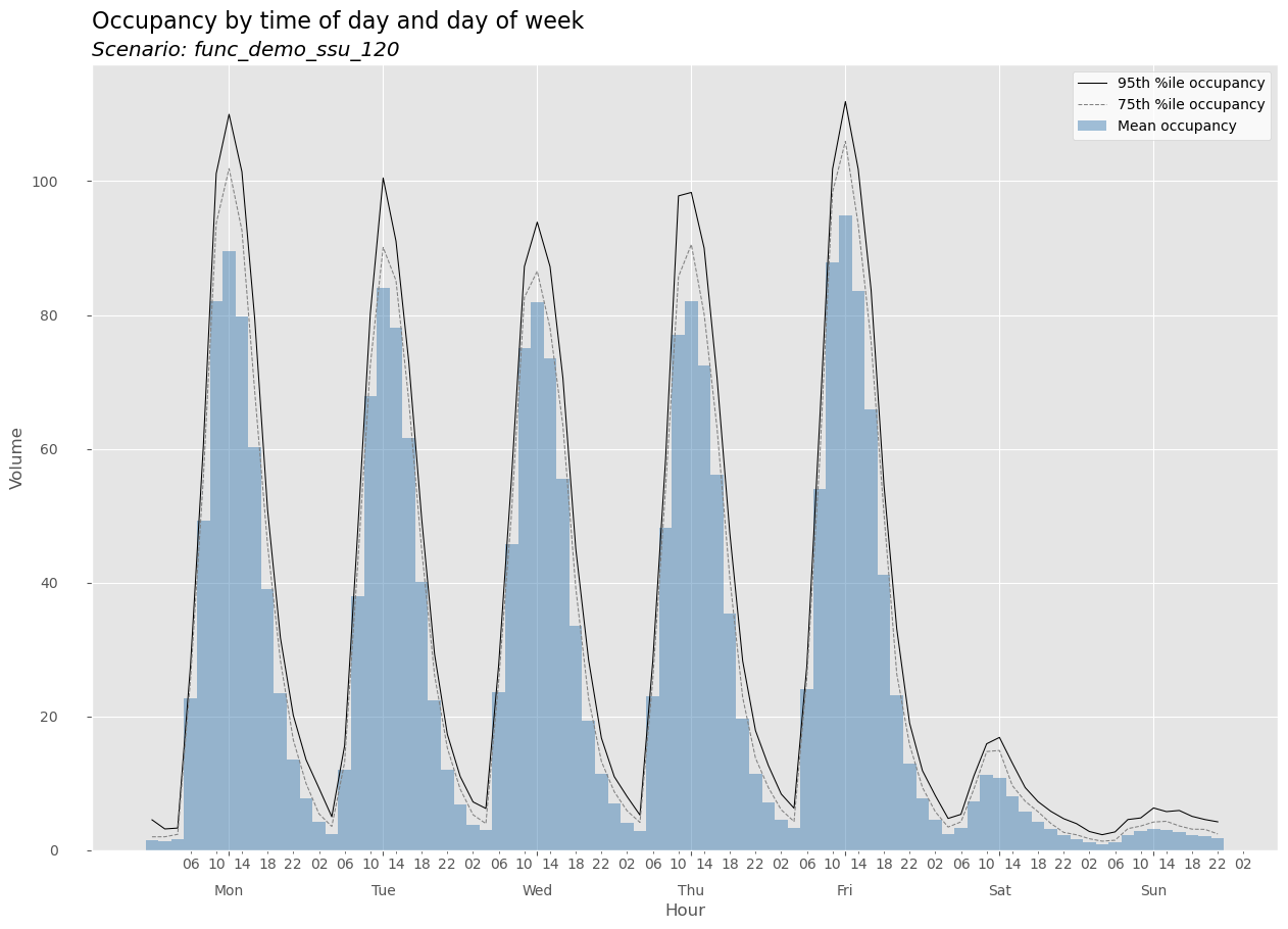
This histogram looks “blockier” due to the two-hour bin sizes.
Using the object oriented hillmaker API#
For more control over hillmaker you can use the object oriented API. In this tutorial we’ll just do a brief introduction. You can get more details in Using object oriented API.
The main steps in using the API are:
create a
Scenarioobject initialized with your hillmaker inputs,call the
make_hillsmethod to run hillmaker and store the outputs in theScenarioobject,use methods to retrieve
Dataframeobjects, plots and other outputs
Here’s a brief example. We’ll use the same inputs as in the first example, except for setting bin_size_minutes=30. By default, plots aren’t automatically created or exported. We will use the export_all_week_plots argument to create and export just the weekly plots. There are a number of other input arguments that can be used for more detailed control of the hillmaker analysis process, but we’ll hold off on that for now.
oo_demo_ssu_30 = hm.Scenario(scenario_name='oo_demo_ssu_30',
                             data=stops_df,
                             in_field='InRoomTS',
                             out_field='OutRoomTS',
                             start_analysis_dt='2024-01-02',
                             end_analysis_dt='2024-09-30',
                             cat_field='PatType',
                             bin_size_minutes=30,
                             plot_export_path='./output',
                             export_all_week_plots=True)

# Show datatype
type(oo_demo_ssu_30)
hillmaker.scenario.Scenario
You can see the values for all of the input parameters by printing the scenario object.
print(oo_demo_ssu_30)
Required inputs
-------------------------
scenario_name = oo_demo_ssu_30
data =
       PatID            InRoomTS           OutRoomTS PatType  LOS_hours
0          1 2024-01-01 07:44:00 2024-01-01 09:20:00     IVT   1.600000
1          2 2024-01-01 08:28:00 2024-01-01 11:13:00     IVT   2.750000
2          3 2024-01-01 11:44:00 2024-01-01 12:48:00     MYE   1.066667
3          4 2024-01-01 11:51:00 2024-01-01 21:10:00     CAT   9.316667
4          5 2024-01-01 12:10:00 2024-01-01 12:57:00     IVT   0.783333
...      ...                 ...                 ...     ...        ...
59872  59873 2024-09-30 19:31:00 2024-09-30 20:34:00     IVT   1.050000
59873  59874 2024-09-30 20:23:00 2024-09-30 22:22:00     IVT   1.983333
59874  59875 2024-09-30 21:00:00 2024-09-30 23:22:00     CAT   2.366667
59875  59876 2024-09-30 21:57:00 2024-10-01 01:58:00     IVT   4.016667
59876  59877 2024-09-30 22:45:00 2024-10-01 03:18:00     CAT   4.550000

[59877 rows x 5 columns]
in_field = InRoomTS
out_field = OutRoomTS
start_analysis_dt = 2024-01-02T00:00:00.000000000
end_analysis_dt = 2024-09-30T23:59:59.000000000

Frequently used optional inputs
-----------------------------------
cat_field = PatType
bin_size_minutes = 30

More optional inputs
-------------------------
cats_to_exclude = None
occ_weight_field = None
percentiles = (0.25, 0.5, 0.75, 0.95, 0.99)
los_units = hours

Dataframe export options
-------------------------
export_bydatetime_csv = False
export_summaries_csv = False
csv_export_path = .

Macro-level plot options
-------------------------
make_all_dow_plots = False
make_all_week_plots = True
export_all_dow_plots = False
export_all_week_plots = True
plot_export_path = ./output

Micro-level plot options
-------------------------
plot_style = ggplot
figsize = (15, 10)
bar_color_mean = steelblue
plot_percentiles = (0.95, 0.75)
pctile_color = ('black', 'grey')
pctile_linestyle = ('-', '--')
pctile_linewidth = (0.75, 0.75)
cap = None
cap_color = r
xlabel = Hour
ylabel = Volume
main_title =
main_title_properties = {'loc': 'left', 'fontsize': 16}
subtitle =
subtitle_properties = {'loc': 'left', 'style': 'italic'}
legend_properties = {'loc': 'best', 'frameon': True, 'facecolor': 'w'}
first_dow = mon

Advanced options
-------------------------
edge_bins = 1
highres_bin_size_minutes = 30
keep_highres_bydatetime = False
nonstationary_stats = True
stationary_stats = True
verbosity = 0
Let’s make some hills. By default, the verbosity parameter is set to 0 - we won’t get any messages unless they are warnings or errors.
oo_demo_ssu_30.make_hills()
All of the outputs from running make_hills get stored in an attribute dictionary called hills.
oo_demo_ssu_30.hills.keys()
dict_keys(['bydatetime', 'summaries', 'los_summary', 'settings', 'plots', 'runtime'])
There are methods for retrieving specific items from this dictionary. For example, there is get_plot.
help(oo_demo_ssu_30.get_plot)
Help on method get_plot in module hillmaker.scenario:

get_plot(flow_metric: str = 'occupancy', day_of_week: str = 'week') method of hillmaker.scenario.Scenario instance
    Get plot object for specified flow metric and whether full week or specified day of week.

    Parameters
    ----------
    flow_metric : str
        Either of 'arrivals', 'departures', 'occupancy' ('a', 'd', and 'o' are sufficient).
        Default='occupancy'
    day_of_week : str
        Either of 'week', 'Sun', 'Mon', 'Tue', 'Wed', 'Thu', 'Fri', 'Sat'. Default='week'

    Returns
    -------
    plot object from matplotlib
oo_demo_ssu_30.get_plot('occupancy')

Similarly, we can use get_bydatetime_df and get_summary to get at specific results DataFrame objects.
help(oo_demo_ssu_30.get_bydatetime_df)
Help on method get_bydatetime_df in module hillmaker.scenario:

get_bydatetime_df(by_category: bool = True) method of hillmaker.scenario.Scenario instance
    Get bydatetime dataframe

    Parameters
    ----------
    by_category : bool
        Default=True corresponds to category specific statistics. A value of False gives overall statistics.


    Returns
    -------
    DataFrame
oo_demo_ssu_30.get_bydatetime_df(by_category=False)
| arrivals | departures | occupancy | day_of_week | dow_name | bin_of_day_str | bin_of_day | bin_of_week | |
|---|---|---|---|---|---|---|---|---|
| datetime | ||||||||
| 2024-01-02 00:00:00 | 0.0 | 0.0 | 1.000000 | 1 | Tue | 00:00 | 0 | 48 |
| 2024-01-02 00:30:00 | 0.0 | 0.0 | 1.000000 | 1 | Tue | 00:30 | 1 | 49 |
| 2024-01-02 01:00:00 | 0.0 | 0.0 | 1.000000 | 1 | Tue | 01:00 | 2 | 50 |
| 2024-01-02 01:30:00 | 0.0 | 1.0 | 0.766667 | 1 | Tue | 01:30 | 3 | 51 |
| 2024-01-02 02:00:00 | 0.0 | 0.0 | 0.000000 | 1 | Tue | 02:00 | 4 | 52 |
| ... | ... | ... | ... | ... | ... | ... | ... | ... |
| 2024-09-30 21:30:00 | 1.0 | 7.0 | 19.700000 | 0 | Mon | 21:30 | 43 | 43 |
| 2024-09-30 22:00:00 | 0.0 | 3.0 | 15.366667 | 0 | Mon | 22:00 | 44 | 44 |
| 2024-09-30 22:30:00 | 1.0 | 4.0 | 11.433333 | 0 | Mon | 22:30 | 45 | 45 |
| 2024-09-30 23:00:00 | 0.0 | 2.0 | 10.333333 | 0 | Mon | 23:00 | 46 | 46 |
| 2024-09-30 23:30:00 | 0.0 | 4.0 | 6.766667 | 0 | Mon | 23:30 | 47 | 47 |
13104 rows × 8 columns
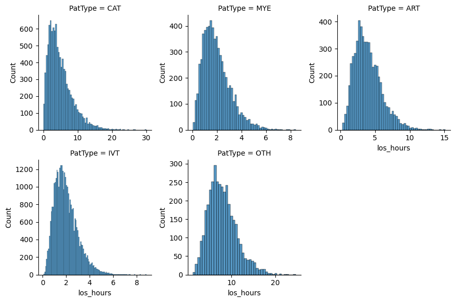
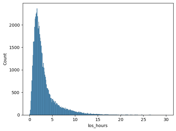
You may have noticed that there were a few other keys in the hills dictionary. For example, we can get a simple length of stay summary. The summary is comprised of two histogram plots and two tabular summaries - one each that are by category and one that is aggregated over all records in the stop data.
oo_demo_ssu_30.hills['los_summary']
{'los_stats': <pandas.io.formats.style.Styler at 0x7f758d29d150>,
 'los_histo': <Figure size 640x480 with 1 Axes>,
 'los_stats_bycat': <pandas.io.formats.style.Styler at 0x7f7587afc1f0>,
 'los_histo_bycat': <Figure size 900x600 with 5 Axes>}
oo_demo_ssu_30.get_los_plot()
oo_demo_ssu_30.get_los_plot(by_category=False)
oo_demo_ssu_30.get_los_stats()
| count | mean | min | max | stdev | cv | skew | p50 | p75 | p95 | p99 | |
|---|---|---|---|---|---|---|---|---|---|---|---|
| PatType | |||||||||||
| ART | 5761 | 4.0 | 0.3 | 15.1 | 2.0 | 0.5 | 1.0 | 3.7 | 5.1 | 7.7 | 9.9 |
| CAT | 10691 | 4.9 | 0.0 | 30.1 | 3.5 | 0.7 | 1.3 | 4.1 | 6.7 | 11.8 | 16.2 |
| IVT | 33174 | 2.0 | 0.1 | 8.8 | 1.0 | 0.5 | 1.0 | 1.8 | 2.5 | 3.9 | 5.0 |
| MYE | 6477 | 2.0 | 0.1 | 8.4 | 1.1 | 0.6 | 1.0 | 1.8 | 2.6 | 4.2 | 5.4 |
| OTH | 3767 | 7.9 | 1.2 | 24.7 | 3.2 | 0.4 | 0.8 | 7.5 | 9.8 | 14.1 | 17.2 |
oo_demo_ssu_30.get_los_stats(by_category=False)
| count | mean | min | max | stdev | cv | skew | p50 | p75 | p95 | p99 | |
|---|---|---|---|---|---|---|---|---|---|---|---|
| all | 59870 | 3.1 | 0.0 | 30.1 | 2.6 | 0.9 | 2.3 | 2.2 | 3.7 | 8.7 | 13.2 |
See Using object oriented API for all the details on using the API.