Using object oriented API

import pandas as pd
import hillmaker as hm

An OO version of hillmaker

Recently, an object oriented API was added to hillmaker to allow analysts to have finer control over the analysis process. Some of the features and architectural details include:

• a Scenario class which has methods for running hillmaker (make_hills()) and for retrieving plots and dataframes from the results dictionary (get_plot(), get_summary_df(), and get_bydatetime_df()).

• the plots and dataframes produced by make_hills() are stored in a dictionary called hills that is an attribute of the Scenario class.

• the methods of the Scenario class are just wrappers that call module level functions of the same name that do the actual work. By doing this, we kept the legacy function interface described in Using the make_hills() function.

• the Scenario class is actually a pydantic model which handles input validation.

The example scenario

Again, we’ll use the Short Stay Unit data for this tutorial.

ssu_stopdata = 'https://raw.githubusercontent.com/misken/hillmaker-examples/main/data/ssu_2024.csv'
# ssu_stopdata = './data/ssu_2024.csv'
ssu_stops_df = pd.read_csv(ssu_stopdata, parse_dates=['InRoomTS','OutRoomTS'])
ssu_stops_df.info() # Check out the structure of the resulting DataFrame

<class 'pandas.core.frame.DataFrame'>
RangeIndex: 59877 entries, 0 to 59876
Data columns (total 5 columns):
 #   Column     Non-Null Count  Dtype         
---  ------     --------------  -----         
 0   PatID      59877 non-null  int64         
 1   InRoomTS   59877 non-null  datetime64[ns]
 2   OutRoomTS  59877 non-null  datetime64[ns]
 3   PatType    59877 non-null  object        
 4   LOS_hours  59877 non-null  float64       
dtypes: datetime64[ns](2), float64(1), int64(1), object(1)
memory usage: 2.3+ MB

The Scenario class

The Scenario class is a pydantic model. It handles a bunch of type constraints, validation, and default values.

We can create scenarios a few different ways.

• instantiate an instance of Scenario by passing in keyword arguments,

• there’s a create_scenario function that can take any or all of a dictionary, a TOML path or keyword argurments and returns a Scenario object (precedence is in the reverse order - kwargs get the final say).

Create a new scenario with keyword arguments

You can create an instance of Scenario by passing in keyword arguments.

Here are a collection of inputs that we’ll use to create a scenario. Notice we purposely set one of the input dates to a string and the other to a Timestamp just to show that the pydantic model can handle the automatic transformation for us to a datetime.

# Required inputs
scenario_name = 'ssu_oo_1'
stops_df = ssu_stops_df
in_field_name = 'InRoomTS'
out_field_name = 'OutRoomTS'
start_date = '2024-06-01'
end_date = pd.Timestamp('8/31/2024')

# Optional inputs
cat_field_name = 'PatType'
bin_size_minutes = 60

scenario_1 = hm.Scenario(scenario_name=scenario_name, 
                         data=stops_df,
                         in_field=in_field_name,
                         out_field=out_field_name,
                         start_analysis_dt=start_date,
                         end_analysis_dt=end_date,
                         cat_field=cat_field_name,
                         bin_size_minutes=bin_size_minutes)

print(scenario_1)

Required inputs
-------------------------
scenario_name = ssu_oo_1
data =
       PatID            InRoomTS           OutRoomTS PatType  LOS_hours
0          1 2024-01-01 07:44:00 2024-01-01 09:20:00     IVT   1.600000
1          2 2024-01-01 08:28:00 2024-01-01 11:13:00     IVT   2.750000
2          3 2024-01-01 11:44:00 2024-01-01 12:48:00     MYE   1.066667
3          4 2024-01-01 11:51:00 2024-01-01 21:10:00     CAT   9.316667
4          5 2024-01-01 12:10:00 2024-01-01 12:57:00     IVT   0.783333
...      ...                 ...                 ...     ...        ...
59872  59873 2024-09-30 19:31:00 2024-09-30 20:34:00     IVT   1.050000
59873  59874 2024-09-30 20:23:00 2024-09-30 22:22:00     IVT   1.983333
59874  59875 2024-09-30 21:00:00 2024-09-30 23:22:00     CAT   2.366667
59875  59876 2024-09-30 21:57:00 2024-10-01 01:58:00     IVT   4.016667
59876  59877 2024-09-30 22:45:00 2024-10-01 03:18:00     CAT   4.550000

[59877 rows x 5 columns]
in_field = InRoomTS
out_field = OutRoomTS
start_analysis_dt = 2024-06-01T00:00:00.000000000
end_analysis_dt = 2024-08-31T23:59:59.000000000

Frequently used optional inputs
-----------------------------------
cat_field = PatType
bin_size_minutes = 60

More optional inputs
-------------------------
cats_to_exclude = None
occ_weight_field = None
percentiles = (0.25, 0.5, 0.75, 0.95, 0.99)
los_units = hours

Dataframe export options
-------------------------
export_bydatetime_csv = False
export_summaries_csv = False
csv_export_path = .

Macro-level plot options
-------------------------
make_all_dow_plots = False
make_all_week_plots = True
export_all_dow_plots = False
export_all_week_plots = False
plot_export_path = None

Micro-level plot options
-------------------------
plot_style = ggplot
figsize = (15, 10)
bar_color_mean = steelblue
plot_percentiles = (0.95, 0.75)
pctile_color = ('black', 'grey')
pctile_linestyle = ('-', '--')
pctile_linewidth = (0.75, 0.75)
cap = None
cap_color = r
xlabel = Hour
ylabel = Volume
main_title = 
main_title_properties = {'loc': 'left', 'fontsize': 16}
subtitle = 
subtitle_properties = {'loc': 'left', 'style': 'italic'}
legend_properties = {'loc': 'best', 'frameon': True, 'facecolor': 'w'}
first_dow = mon

Advanced options
-------------------------
edge_bins = 1
highres_bin_size_minutes = 60
keep_highres_bydatetime = False
nonstationary_stats = True
stationary_stats = True
verbosity = 0

Now use the make_hills method to run hillmaker.

scenario_1.make_hills()

By default, only weekly plots are created - make_all_dow_plots defaults to False and make_all_week_plots defaults to True.

scenario_1.hills.keys()

dict_keys(['bydatetime', 'summaries', 'los_summary', 'settings', 'plots', 'runtime'])

summary_df = scenario_1.get_summary_df(by_category=False)
summary_df

	day_of_week	dow_name	bin_of_day	bin_of_day_str	count	mean	min	max	stdev	sem	var	cv	skew	kurt	p25	p50	p75	p95	p99
0	0	Mon	0	00:00	13.0	1.001282	0.0	3.000000	0.923396	0.256104	0.852660	0.922214	0.789389	0.158285	0.250000	1.000000	1.450000	2.400000	2.880000
1	0	Mon	1	01:00	13.0	0.980769	0.0	2.600000	0.756724	0.209878	0.572632	0.771562	0.582793	0.606338	0.750000	1.000000	1.133333	2.240000	2.528000
2	0	Mon	2	02:00	13.0	0.734615	0.0	1.866667	0.628802	0.174398	0.395392	0.855961	0.026817	-1.153303	0.000000	1.000000	1.000000	1.546667	1.802667
3	0	Mon	3	03:00	13.0	0.598718	0.0	1.733333	0.604093	0.167545	0.364929	1.008978	0.269351	-1.274639	0.000000	1.000000	1.000000	1.303333	1.647333
4	0	Mon	4	04:00	13.0	0.539744	0.0	2.000000	0.633536	0.175711	0.401368	1.173772	0.988444	0.557461	0.000000	0.300000	1.000000	1.400000	1.880000
...	...	...	...	...	...	...	...	...	...	...	...	...	...	...	...	...	...	...	...
163	6	Sun	19	19:00	13.0	1.885897	0.0	5.400000	1.417367	0.393107	2.008928	0.751561	1.077564	2.303828	1.000000	2.000000	2.116667	3.970000	5.114000
164	6	Sun	20	20:00	13.0	1.603846	0.0	4.000000	1.100550	0.305238	1.211211	0.686194	0.580109	0.805758	1.000000	1.683333	2.016667	3.390000	3.878000
165	6	Sun	21	21:00	13.0	1.730769	0.0	4.466667	1.170803	0.324722	1.370780	0.676464	0.992959	1.212156	1.000000	1.266667	2.466667	3.586667	4.290667
166	6	Sun	22	22:00	13.0	1.352564	0.0	4.066667	1.117347	0.309896	1.248465	0.826096	1.309961	2.012192	1.000000	1.016667	1.666667	3.366667	3.926667
167	6	Sun	23	23:00	13.0	1.251282	0.0	3.550000	1.017041	0.282077	1.034373	0.812799	0.783495	0.929374	0.933333	1.000000	1.516667	2.890000	3.418000

168 rows × 19 columns

summary_df[summary_df['dow_name']=='Mon']

	day_of_week	dow_name	bin_of_day	bin_of_day_str	count	mean	min	max	stdev	sem	var	cv	skew	kurt	p25	p50	p75	p95	p99
0	0	Mon	0	00:00	13.0	1.001282	0.000000	3.000000	0.923396	0.256104	0.852660	0.922214	0.789389	0.158285	0.250000	1.000000	1.450000	2.400000	2.880000
1	0	Mon	1	01:00	13.0	0.980769	0.000000	2.600000	0.756724	0.209878	0.572632	0.771562	0.582793	0.606338	0.750000	1.000000	1.133333	2.240000	2.528000
2	0	Mon	2	02:00	13.0	0.734615	0.000000	1.866667	0.628802	0.174398	0.395392	0.855961	0.026817	-1.153303	0.000000	1.000000	1.000000	1.546667	1.802667
3	0	Mon	3	03:00	13.0	0.598718	0.000000	1.733333	0.604093	0.167545	0.364929	1.008978	0.269351	-1.274639	0.000000	1.000000	1.000000	1.303333	1.647333
4	0	Mon	4	04:00	13.0	0.539744	0.000000	2.000000	0.633536	0.175711	0.401368	1.173772	0.988444	0.557461	0.000000	0.300000	1.000000	1.400000	1.880000
5	0	Mon	5	05:00	13.0	1.738462	0.083333	4.016667	1.221895	0.338893	1.493027	0.702860	0.719157	-0.067127	0.750000	1.566667	2.183333	3.946667	4.002667
6	0	Mon	6	06:00	13.0	15.611538	12.933333	21.483333	2.253489	0.625005	5.078212	0.144348	1.536775	2.969572	14.400000	14.816667	17.083333	19.053333	20.997333
7	0	Mon	7	07:00	13.0	30.598718	23.833333	35.350000	3.758518	1.042425	14.126457	0.122833	-0.201338	-1.089779	28.100000	29.683333	33.650000	35.260000	35.332000
8	0	Mon	8	08:00	13.0	40.041026	28.866667	50.250000	6.065978	1.682400	36.796093	0.151494	-0.169844	-0.525927	35.300000	40.783333	44.816667	47.940000	49.788000
9	0	Mon	9	09:00	13.0	60.360256	46.600000	74.366667	7.248399	2.010344	52.539284	0.120086	0.227562	0.324710	56.900000	57.983333	64.916667	71.056667	73.704667
10	0	Mon	10	10:00	13.0	79.779487	65.600000	92.483333	8.066868	2.237347	65.074359	0.101115	-0.088912	-0.401957	73.683333	80.366667	85.050000	92.213333	92.429333
11	0	Mon	11	11:00	13.0	90.783333	69.483333	104.566667	10.433342	2.893688	108.854630	0.114926	-0.628558	0.012274	87.000000	91.550000	96.616667	103.966667	104.446667
12	0	Mon	12	12:00	13.0	94.185897	76.783333	112.500000	11.018183	3.055894	121.400363	0.116983	-0.190239	-0.795746	87.383333	96.550000	101.350000	108.510000	111.702000
13	0	Mon	13	13:00	13.0	93.706410	71.833333	105.483333	11.381087	3.156546	129.529145	0.121455	-0.635205	-1.027072	83.966667	97.816667	101.700000	105.403333	105.467333
14	0	Mon	14	14:00	13.0	89.667949	68.816667	105.366667	11.253657	3.121203	126.644790	0.125504	-0.488596	-0.771888	80.983333	89.900000	99.433333	102.826667	104.858667
15	0	Mon	15	15:00	13.0	83.123077	63.200000	98.066667	11.043608	3.062946	121.961275	0.132859	-0.582014	-0.471980	77.233333	82.700000	90.300000	96.946667	97.842667
16	0	Mon	16	16:00	13.0	72.489744	53.283333	89.616667	11.459360	3.178255	131.316923	0.158082	-0.015937	-0.915821	65.816667	70.783333	81.883333	89.266667	89.546667
17	0	Mon	17	17:00	13.0	59.478205	43.700000	74.916667	9.724336	2.697045	94.562703	0.163494	0.005002	-0.481753	55.000000	58.033333	64.416667	74.176667	74.768667
18	0	Mon	18	18:00	13.0	47.285897	34.416667	59.950000	7.971369	2.210860	63.542724	0.168578	-0.060306	-1.058324	42.233333	48.983333	52.666667	58.280000	59.616000
19	0	Mon	19	19:00	13.0	36.300000	25.616667	54.766667	8.557209	2.373343	73.225833	0.235736	0.713560	-0.016054	30.500000	32.666667	41.783333	48.976667	53.608667
20	0	Mon	20	20:00	13.0	28.357692	19.633333	43.683333	7.511431	2.083296	56.421603	0.264882	0.593998	-0.619724	22.866667	24.150000	33.816667	38.663333	42.679333
21	0	Mon	21	21:00	13.0	21.889744	13.800000	32.533333	6.060056	1.680757	36.724284	0.276845	0.257447	-1.137251	17.600000	22.150000	25.883333	30.743333	32.175333
22	0	Mon	22	22:00	13.0	17.144872	9.400000	24.483333	4.657751	1.291828	21.694647	0.271670	-0.112883	-0.264315	14.966667	17.516667	19.100000	24.413333	24.469333
23	0	Mon	23	23:00	13.0	13.453846	5.750000	19.833333	4.543550	1.260154	20.643850	0.337714	-0.328681	-0.905871	10.083333	13.483333	17.966667	19.013333	19.669333

Plots can be retrieved with the get_plot() method.

scenario_1.get_plot('occ')

scenario_1.get_plot('arrivals')

If you prefer, you can also use the compute_hills_stats() method which will not create any plots. We’ll create a new scenario that uses a smaller bins size.

scenario_1a = hm.Scenario(scenario_name='ssu_oo_1a', 
                         data=stops_df,
                         in_field=in_field_name,
                         out_field=out_field_name,
                         start_analysis_dt=start_date,
                         end_analysis_dt=end_date,
                         cat_field=cat_field_name,
                         bin_size_minutes=30)

scenario_1a.compute_hills_stats()

scenario_1a.hills.keys()

dict_keys(['bydatetime', 'summaries', 'los_summary', 'settings'])

Then later, if we decide to generate plots, we can.

help(scenario_1a.make_weekly_plot)

Help on method make_weekly_plot in module hillmaker.scenario:

make_weekly_plot(metric: str = 'occupancy', **kwargs) method of hillmaker.scenario.Scenario instance
    Create weekly plot
    
    Parameters
    ----------
    metric : str
        Some abbreviated version of occupancy, arrivals or departures
    kwargs : dict
        Plot related keyword arguments
    
    Returns
    -------
    matplotlib.Figure
    
    Example
    -------
    scenario_1.make_weekly_plot(metric='occupancy', plot_export_path='./output', cap=40, plot_style='default')

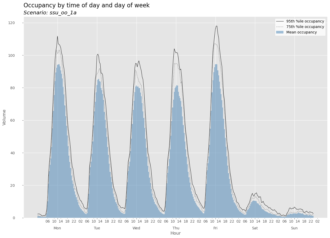
scenario_1a.make_weekly_plot()

If we provide plot_export_path, the plot will get exported as a PNG file.

arrivals_plot = scenario_1a.make_weekly_plot(metric='Arrivals', plot_export_path='./output/')
arrivals_plot

You can use any of the plot related input parameters to style the plot.

scenario_1a.make_weekly_plot(plot_style='classic')

scenario_1a.make_weekly_plot(cap=100, cap_color='blue', bar_color_mean='#ffbb11',
                            ylabel='Patients')

Create scenario from a config file

To use a TOML configuration file to create a scenario, we can use the create_scenario function.

Here’s what an example config file might look like. The scenario_name and bin_size_minutes have been changed from the first scenario in this notebook.

[scenario_data]
scenario_name = "ss_oo_2"
data = "./data/ssu_2024.csv"

[fields]
in_field = "InRoomTS"
out_field = "OutRoomTS"
# Just remove the following line if no category field
cat_field = "PatType"

[analysis_dates]
start_analysis_dt = 2024-01-02
end_analysis_dt = 2024-03-30

[settings]
bin_size_minutes = 120
verbosity = 1
csv_export_path = './output'
plot_export_path = './output'

# Add any additional arguments here
# Strings should be surrounded in double quotes
# Floats and ints are specified in the normal way as values
# Dates are specified as shown above

# For arguments that take lists, the entries look
# just like Python lists and following the other rules above

# cats_to_exclude = ["IVT", "OTH"]
# percentiles = [0.5, 0.8, 0.9]

# For arguments that take dictionaries, do this:
# main_title_properties = {loc = 'left', fontsize = 16}
# subtitle_properties = {loc = 'left', style = 'italic'}
# legend_properties = {loc = 'best', frameon = true, facecolor = 'w'}

The sections headings, [scenario_data], [fields], and [analysis_dates] aren’t actually necessary. You could actually put all input parameters within the [settings] section. Including the other headings is just an organizational aid.

Warning

You MUST include at least the [settings] section header.

help(hm.create_scenario)

Help on function create_scenario in module hillmaker.scenario:

create_scenario(params_dict: Optional[Dict] = None, config_path: Union[str, pathlib.Path, NoneType] = None, **kwargs)
    Function to create a `Scenario` from a dict, a TOML config file, and/or keyword args

From the help() we see that there are three ways to pass input parameters into the create_scenario() function. If you specify a config_path, any inputs set via the config file will override values previously set with the params_dict dictionary. Similarly, any inputs set via **kwargs will override any set via params_dict or config_path.

scenario_2 = hm.create_scenario(config_path='./input/ssu_oo_2.toml')

print(scenario_2)

Required inputs
-------------------------
scenario_name = ss_oo_2
data =
       PatID            InRoomTS           OutRoomTS PatType  LOS_hours
0          1 2024-01-01 07:44:00 2024-01-01 09:20:00     IVT   1.600000
1          2 2024-01-01 08:28:00 2024-01-01 11:13:00     IVT   2.750000
2          3 2024-01-01 11:44:00 2024-01-01 12:48:00     MYE   1.066667
3          4 2024-01-01 11:51:00 2024-01-01 21:10:00     CAT   9.316667
4          5 2024-01-01 12:10:00 2024-01-01 12:57:00     IVT   0.783333
...      ...                 ...                 ...     ...        ...
59872  59873 2024-09-30 19:31:00 2024-09-30 20:34:00     IVT   1.050000
59873  59874 2024-09-30 20:23:00 2024-09-30 22:22:00     IVT   1.983333
59874  59875 2024-09-30 21:00:00 2024-09-30 23:22:00     CAT   2.366667
59875  59876 2024-09-30 21:57:00 2024-10-01 01:58:00     IVT   4.016667
59876  59877 2024-09-30 22:45:00 2024-10-01 03:18:00     CAT   4.550000

[59877 rows x 5 columns]
in_field = InRoomTS
out_field = OutRoomTS
start_analysis_dt = 2024-01-02T00:00:00.000000000
end_analysis_dt = 2024-03-30T23:59:59.000000000

Frequently used optional inputs
-----------------------------------
cat_field = PatType
bin_size_minutes = 120

More optional inputs
-------------------------
cats_to_exclude = None
occ_weight_field = None
percentiles = (0.25, 0.5, 0.75, 0.95, 0.99)
los_units = hours

Dataframe export options
-------------------------
export_bydatetime_csv = False
export_summaries_csv = False
csv_export_path = ./output

Macro-level plot options
-------------------------
make_all_dow_plots = False
make_all_week_plots = True
export_all_dow_plots = False
export_all_week_plots = False
plot_export_path = ./output

Micro-level plot options
-------------------------
plot_style = ggplot
figsize = (15, 10)
bar_color_mean = steelblue
plot_percentiles = (0.95, 0.75)
pctile_color = ('black', 'grey')
pctile_linestyle = ('-', '--')
pctile_linewidth = (0.75, 0.75)
cap = None
cap_color = r
xlabel = Hour
ylabel = Volume
main_title = 
main_title_properties = {'loc': 'left', 'fontsize': 16}
subtitle = 
subtitle_properties = {'loc': 'left', 'style': 'italic'}
legend_properties = {'loc': 'best', 'frameon': True, 'facecolor': 'w'}
first_dow = mon

Advanced options
-------------------------
edge_bins = 1
highres_bin_size_minutes = 120
keep_highres_bydatetime = False
nonstationary_stats = True
stationary_stats = True
verbosity = 1

Create a new scenario using create_scenario() and a dictionary

The create_scenario function also can take, as input, a dictionary of input arguments. Notice in the example below that strings are used for the dates but they just as well could be datetime or TimeStamp objects - anything that can be converted to a pandas TimeStamp is allowed. I’ve only included the required parameters and two optional parameters - cat_field and bin_size_mins.

ssu_oo_3_dict = {
    'scenario_name': 'ssu_oo_3',
    'stops_df': ssu_stops_df,
    'in_field': 'InRoomTS',
    'out_field': 'OutRoomTS',
    'start_analysis_dt': '2024-01-01',
    'end_analysis_dt': '2024-09-30',
    'cat_field': 'PatType',
    'bin_size_minutes': 60
}

ssu_oo_3_dict = {
    'scenario_name': 'ssu_oo_3',
    'data': ssu_stops_df,
    'in_field': 'InRoomTS',
    'out_field': 'OutRoomTS',
    'start_analysis_dt': '2024-01-01',
    'end_analysis_dt': '2024-09-30',
    'cat_field': 'PatType',
    'bin_size_minutes': 60
}

ssu_oo_3 = hm.create_scenario(params_dict=ssu_oo_3_dict)
print(ssu_oo_3)

Required inputs
-------------------------
scenario_name = ssu_oo_3
data =
       PatID            InRoomTS           OutRoomTS PatType  LOS_hours
0          1 2024-01-01 07:44:00 2024-01-01 09:20:00     IVT   1.600000
1          2 2024-01-01 08:28:00 2024-01-01 11:13:00     IVT   2.750000
2          3 2024-01-01 11:44:00 2024-01-01 12:48:00     MYE   1.066667
3          4 2024-01-01 11:51:00 2024-01-01 21:10:00     CAT   9.316667
4          5 2024-01-01 12:10:00 2024-01-01 12:57:00     IVT   0.783333
...      ...                 ...                 ...     ...        ...
59872  59873 2024-09-30 19:31:00 2024-09-30 20:34:00     IVT   1.050000
59873  59874 2024-09-30 20:23:00 2024-09-30 22:22:00     IVT   1.983333
59874  59875 2024-09-30 21:00:00 2024-09-30 23:22:00     CAT   2.366667
59875  59876 2024-09-30 21:57:00 2024-10-01 01:58:00     IVT   4.016667
59876  59877 2024-09-30 22:45:00 2024-10-01 03:18:00     CAT   4.550000

[59877 rows x 5 columns]
in_field = InRoomTS
out_field = OutRoomTS
start_analysis_dt = 2024-01-01T00:00:00.000000000
end_analysis_dt = 2024-09-30T23:59:59.000000000

Frequently used optional inputs
-----------------------------------
cat_field = PatType
bin_size_minutes = 60

More optional inputs
-------------------------
cats_to_exclude = None
occ_weight_field = None
percentiles = (0.25, 0.5, 0.75, 0.95, 0.99)
los_units = hours

Dataframe export options
-------------------------
export_bydatetime_csv = False
export_summaries_csv = False
csv_export_path = .

Macro-level plot options
-------------------------
make_all_dow_plots = False
make_all_week_plots = True
export_all_dow_plots = False
export_all_week_plots = False
plot_export_path = None

Micro-level plot options
-------------------------
plot_style = ggplot
figsize = (15, 10)
bar_color_mean = steelblue
plot_percentiles = (0.95, 0.75)
pctile_color = ('black', 'grey')
pctile_linestyle = ('-', '--')
pctile_linewidth = (0.75, 0.75)
cap = None
cap_color = r
xlabel = Hour
ylabel = Volume
main_title = 
main_title_properties = {'loc': 'left', 'fontsize': 16}
subtitle = 
subtitle_properties = {'loc': 'left', 'style': 'italic'}
legend_properties = {'loc': 'best', 'frameon': True, 'facecolor': 'w'}
first_dow = mon

Advanced options
-------------------------
edge_bins = 1
highres_bin_size_minutes = 60
keep_highres_bydatetime = False
nonstationary_stats = True
stationary_stats = True
verbosity = 0

With create_scenario, you can also include keyword arguments that will take precedence over those specified in either a TOML file or a dictionary.

ssu_oo_3 = hm.create_scenario(params_dict=ssu_oo_3_dict, 
                              export_summaries_csv=True, csv_export_path='./output',
                              bin_size_minutes=30)

print(ssu_oo_3.export_summaries_csv)
print(ssu_oo_3.bin_size_minutes)

True
30

Now let’s generate hills by using the make_hills method of one of the scenario instances.

ssu_oo_3.make_hills()

We can use the get_summary_df() method to retrieve summary dataframes.

help(ssu_oo_3.get_summary_df)

Help on method get_summary_df in module hillmaker.scenario:

get_summary_df(flow_metric: str = 'occupancy', by_category: bool = True, stationary: bool = False) method of hillmaker.scenario.Scenario instance
    Get summary dataframe
    
    Parameters
    ----------
    flow_metric : str
        Either of 'arrivals', 'departures', 'occupancy' ('a', 'd', and 'o' are sufficient).
        Default='occupancy'
    by_category : bool
        Default=True corresponds to category specific statistics. A value of False gives overall statistics.
    stationary : bool
        Default=False corresponds to the standard nonstationary statistics (i.e. by TOD and DOW)
    
    Returns
    -------
    DataFrame

ssu_oo_3.get_summary_df()

	PatType	day_of_week	dow_name	bin_of_day	bin_of_day_str	count	mean	min	max	stdev	sem	var	cv	skew	kurt	p25	p50	p75	p95	p99
0	ART	0	Mon	0	00:00	40.0	0.0	0.0	0.0	0.0	0.0	0.0	0.0	0.0	0.0	0.0	0.0	0.0	0.0	0.0
1	ART	0	Mon	1	00:30	40.0	0.0	0.0	0.0	0.0	0.0	0.0	0.0	0.0	0.0	0.0	0.0	0.0	0.0	0.0
2	ART	0	Mon	2	01:00	40.0	0.0	0.0	0.0	0.0	0.0	0.0	0.0	0.0	0.0	0.0	0.0	0.0	0.0	0.0
3	ART	0	Mon	3	01:30	40.0	0.0	0.0	0.0	0.0	0.0	0.0	0.0	0.0	0.0	0.0	0.0	0.0	0.0	0.0
4	ART	0	Mon	4	02:00	40.0	0.0	0.0	0.0	0.0	0.0	0.0	0.0	0.0	0.0	0.0	0.0	0.0	0.0	0.0
...	...	...	...	...	...	...	...	...	...	...	...	...	...	...	...	...	...	...	...	...
1675	OTH	6	Sun	43	21:30	39.0	0.0	0.0	0.0	0.0	0.0	0.0	0.0	0.0	0.0	0.0	0.0	0.0	0.0	0.0
1676	OTH	6	Sun	44	22:00	39.0	0.0	0.0	0.0	0.0	0.0	0.0	0.0	0.0	0.0	0.0	0.0	0.0	0.0	0.0
1677	OTH	6	Sun	45	22:30	39.0	0.0	0.0	0.0	0.0	0.0	0.0	0.0	0.0	0.0	0.0	0.0	0.0	0.0	0.0
1678	OTH	6	Sun	46	23:00	39.0	0.0	0.0	0.0	0.0	0.0	0.0	0.0	0.0	0.0	0.0	0.0	0.0	0.0	0.0
1679	OTH	6	Sun	47	23:30	39.0	0.0	0.0	0.0	0.0	0.0	0.0	0.0	0.0	0.0	0.0	0.0	0.0	0.0	0.0

1680 rows × 20 columns