Using the make_hills() function#
The hillmaker.hills.make_hills function is the gateway to hillmaker and is used by the CLI, the object oriented API, or on its own to launch the hillmaking process. It has numerous input arguments for customizing how hillmaker works. In this tutorial we will describe all of the input arguments and discuss their use. This same information applies to CLI as well as the object oriented API’s Scenario.make_hills method.
import pandas as pd
import hillmaker as hm
ssu_stopdata = 'https://raw.githubusercontent.com/misken/hillmaker-examples/main/data/ssu_2024.csv'
# ssu_stopdata = './data/ssu_2024.csv'
ssu_stops_df = pd.read_csv(ssu_stopdata, parse_dates=['InRoomTS','OutRoomTS'])
ssu_stops_df.info() # Check out the structure of the resulting DataFrame
<class 'pandas.core.frame.DataFrame'>
RangeIndex: 59877 entries, 0 to 59876
Data columns (total 5 columns):
 #   Column     Non-Null Count  Dtype
---  ------     --------------  -----
 0   PatID      59877 non-null  int64
 1   InRoomTS   59877 non-null  datetime64[ns]
 2   OutRoomTS  59877 non-null  datetime64[ns]
 3   PatType    59877 non-null  object
 4   LOS_hours  59877 non-null  float64
dtypes: datetime64[ns](2), float64(1), int64(1), object(1)
memory usage: 2.3+ MB
help(hm.make_hills)
Help on function make_hills in module hillmaker.legacy:

make_hills(scenario_name: str = None, data: str | pathlib.Path | pandas.core.frame.DataFrame = None, in_field: str = None, out_field: str = None, start_analysis_dt: str | datetime.date | datetime.datetime | pandas._libs.tslibs.timestamps.Timestamp | numpy.datetime64 = None, end_analysis_dt: str | datetime.date | datetime.datetime | pandas._libs.tslibs.timestamps.Timestamp | numpy.datetime64 = None, cat_field: str = None, bin_size_minutes: int = 60, export_bydatetime_csv: bool = True, export_summaries_csv: bool = True, csv_export_path: str | pathlib.Path = PosixPath('.'), make_all_dow_plots: bool = True, make_all_week_plots: bool = True, export_all_dow_plots: bool = False, export_all_week_plots: bool = False, plot_export_path: str | pathlib.Path = PosixPath('.'), **kwargs) -> Dict
    Compute occupancy, arrival, and departure statistics by category, time bin of day and day of week.

    Main function that first calls `bydatetime.make_bydatetime` to calculate occupancy, arrival
    and departure values by date by time bin and then calls `summarize.summarize`
    to compute the summary statistics.

    Parameters
    ----------
    scenario_name : str
        Used in output filenames
    data : str, Path, or DataFrame
        Base data containing one row per visit. If Path-like, data is read into a DataFrame.
    in_field : str
        Column name corresponding to the arrival times
    out_field : str
        Column name corresponding to the departure times
    start_analysis_dt : datetime-like, str
        Starting datetime for the analysis (must be convertible to pandas Timestamp)
    end_analysis_dt : datetime-like, str
        Ending datetime for the analysis (must be convertible to pandas Timestamp)
    cat_field : str, optional
        Column name corresponding to the categories. If none is specified, then only overall occupancy is summarized.
        Default is None
    bin_size_minutes : int, optional
        Number of minutes in each time bin of the day, default is 60. This bin size is used for plots and reporting and
        is an aggregation of computations done at the finer bin size resolution specified by `resolution_bin_size_mins`.
        Use a value that divides into 1440 with no remainder.
    cats_to_exclude : list, optional
        Category values to ignore, default is None
    occ_weight_field : str, optional
        Column name corresponding to the weights to use for occupancy incrementing, default is None
        which corresponds to a weight of 1.0
    percentiles : list or tuple of floats (e.g. [0.5, 0.75, 0.95]), optional
        Which percentiles to compute. Default is (0.25, 0.5, 0.75, 0.95, 0.99)
    los_units : str, optional
        The time units for length of stay analysis.
        See https://pandas.pydata.org/docs/reference/api/pandas.Timedelta.html for allowable values (smallest
        value allowed is 'seconds', largest is 'days'). The default is 'hours'.

    export_bydatetime_csv : bool, optional
       If True, bydatetime DataFrames are exported to csv files. Default is False.
    export_summaries_csv : bool, optional
       If True, summary DataFrames are exported to csv files. Default is False.
    csv_export_path : str or Path, optional
        Destination path for exported csv files, default is the current directory

    make_all_dow_plots : bool, optional
       If True, day of week plots are created for occupancy, arrival, and departure. Default is True.
    make_all_week_plots : bool, optional
       If True, full week plots are created for occupancy, arrival, and departure. Default is True.
    export_all_dow_plots : bool, optional
       If True, day of week plots are exported for occupancy, arrival, and departure. Default is False.
    export_all_week_plots : bool, optional
       If True, full week plots are exported for occupancy, arrival, and departure. Default is False.
    plot_export_path : str or Path, optional, default is the current directory
        Destination path for exported png files, default is the current directory

    plot_style : str, optional
        Matplotlib built in style name. Default is 'ggplot'.
    figsize : Tuple, optional
        Figure size. Default is (15, 10)
    bar_color_mean : str, optional
        Matplotlib color name for the bars representing mean values. Default is 'steelblue'
    alpha : float, optional
        Transparency level for bars. Default = 0.5.
    plot_percentiles : list or tuple of floats (e.g. [0.75, 0.95]), optional
        Which percentiles to plot. Default is (0.95)
    pctile_color : list or tuple of color codes (e.g. ['blue', 'green'] or list('gb'), optional
        Line color for each percentile series plotted. Order should match order of percentiles list.
        Default is ('black', 'grey').
    pctile_linestyle : List or tuple of line styles (e.g. ['-', '--']), optional
        Line style for each percentile series plotted. Default is ('-', '--').
    pctile_linewidth : List or tuple of line widths in points (e.g. [1.0, 0.75])
        Line width for each percentile series plotted. Default is (0.75, 0.75).
    cap : int, optional
        Capacity of area being analyzed, default is None
    cap_color : str, optional
        matplotlib color code, default='r'
    xlabel : str, optional
        x-axis label, default='Hour'
    ylabel : str, optional
        y-axis label, default='Patients'
    main_title : str, optional
        Main title for plot, default = '{Occupancy or Arrivals or Departures} by time of day and day of week'
    main_title_properties : None or dict, optional
        Dict of main title properties, default={{'loc': 'left', 'fontsize': 16}}
    subtitle : str, optional
        subtitle for plot, default = 'Scenario: {scenario_name}'
    subtitle_properties : None or dict, optional
        Dict of subtitle properties, default={'loc': 'left', 'style': 'italic'}
    legend_properties : None or dict, optional
        Dict of legend properties, default={{'loc': 'best', 'frameon': True, 'facecolor': 'w'}}
    first_dow : str, optional
        Controls which day of week appears first in plot. One of 'mon', 'tue', 'wed', 'thu', 'fri', 'sat, 'sun'

    edge_bins: int, default 1
        Occupancy contribution method for arrival and departure bins. 1=fractional, 2=entire bin
    highres_bin_size_minutes : int, optional
        Number of minutes in each time bin of the day used for initial computation of the number of arrivals,
        departures, and the occupancy level. This value should be <= `bin_size_minutes`. The shorter the duration of
        stays, the smaller the resolution should be. The current default is 5 minutes.
    keep_highres_bydatetime : bool, optional
        Save the high resolution bydatetime dataframe in hills attribute. Default is False.
    nonstationary_stats : bool, optional
       If True, datetime bin stats are computed. Else, they aren't computed. Default is True
    stationary_stats : bool, optional
       If True, overall, non-time bin dependent, stats are computed. Else, they aren't computed. Default is True
    verbosity : int, optional
        Used to set level in loggers. 0=logging.WARNING (default=0), 1=logging.INFO, 2=logging.DEBUG


    Returns
    -------
    dict of DataFrames and plots
       The bydatetime DataFrames, all summary DataFrames and any plots created.

    Example
    -------
    Use like this::

        # Required inputs
        scenario_name = 'ssu_summer24'
        in_field_name = 'InRoomTS'
        out_field_name = 'OutRoomTS'
        start_date = '2024-06-01'
        end_date = '2024-08-31'

        # Optional inputs
        cat_field_name = 'PatType'
        bin_size_minutes = 30
        csv_export_path = './output'

        # Optional plotting inputs
        plot_export_path = './output'
        plot_style = 'default'
        bar_color_mean = 'grey'
        percentiles = [0.85, 0.95]
        plot_percentiles = [0.95, 0.85]
        pctile_color = ['blue', 'green']
        pctile_linewidth = [0.8, 1.0]
        cap = 110
        cap_color = 'black'
        main_title = 'Occupancy summary'
        main_title_properties = {'loc': 'center', 'fontsize':20}
        subtitle = 'Summer 2024 analysis'
        subtitle_properties = {'loc': 'center'}
        xlabel = ''
        ylabel = 'Patients'

        # Optional plotting related inputs

        # Use legacy function interface
        hills = hm.make_hills(scenario_name=scenario_name, data=ssu_stops_df,
                              in_field=in_field_name, out_field=out_field_name,
                              start_analysis_dt=start_date, end_analysis_dt=end_date,
                              cat_field=cat_field_name,
                              bin_size_minutes=bin_size_minutes,
                              csv_export_path=csv_export_path,
                              plot_export_path=plot_export_path, plot_style = plot_style,
                              percentiles=percentiles, plot_percentiles=plot_percentiles,
                              pctile_color=pctile_color, pctile_linewidth=pctile_linewidth,
                              cap=cap, cap_color=cap_color,
                              main_title=main_title, main_title_properties=main_title_properties,
                              subtitle=subtitle, subtitle_properties=subtitle_properties,
                              xlabel=xlabel, ylabel=ylabel
                             )
Required input arguments#
scenario_name (str)#
This is a string that gets used in a few places:
part of filenames of exported CSV files,
part of filenames of exported plots,
plot subtitle default
Since it gets used in filenames, best to avoid spaces and special characters (other than underscore). Any non-alphanumeric characters other than the underscore will get transformed to underscores.
data (str | Path | DataFrame)#
The data table with each row representing one visit, or stop, by an entity. You can pass a string or a Path object to a CSV file, which will then get read into a pandas DataFrame. Or, you can directly pass in a DataFrame.
For example, in the SSU example, each row is a a patient who visits the short stay unit. In cycle share data, each row might be a rental of a bike for some period of time. Here are the first few records from ssu_stops_df. It is NOT necessary to have a field containing the duration of time that the entity spent in the system (e.g. LOS_hours below). You only need to have fields representing the arrival and departure times from the system - InRoomTS and OutRoomTS in this example.
ssu_stops_df.head()
| PatID | InRoomTS | OutRoomTS | PatType | LOS_hours | |
|---|---|---|---|---|---|
| 0 | 1 | 2024-01-01 07:44:00 | 2024-01-01 09:20:00 | IVT | 1.600000 |
| 1 | 2 | 2024-01-01 08:28:00 | 2024-01-01 11:13:00 | IVT | 2.750000 |
| 2 | 3 | 2024-01-01 11:44:00 | 2024-01-01 12:48:00 | MYE | 1.066667 |
| 3 | 4 | 2024-01-01 11:51:00 | 2024-01-01 21:10:00 | CAT | 9.316667 |
| 4 | 5 | 2024-01-01 12:10:00 | 2024-01-01 12:57:00 | IVT | 0.783333 |
in_field (str)#
The fieldname in data containing the arrival times. The datatype for the field itself must be a pandas Timestamp (or datetime64).
out_field (str)#
The fieldname in data containing the departure times. The datatype for the field itself must be a pandas Timestamp (or datetime64).
ssu_stops_df.info()
<class 'pandas.core.frame.DataFrame'>
RangeIndex: 59877 entries, 0 to 59876
Data columns (total 5 columns):
 #   Column     Non-Null Count  Dtype
---  ------     --------------  -----
 0   PatID      59877 non-null  int64
 1   InRoomTS   59877 non-null  datetime64[ns]
 2   OutRoomTS  59877 non-null  datetime64[ns]
 3   PatType    59877 non-null  object
 4   LOS_hours  59877 non-null  float64
dtypes: datetime64[ns](2), float64(1), int64(1), object(1)
memory usage: 2.3+ MB
start_analysis_dt and end_analysis_dt (something convertible to a pandas Timestamp)#
These two dates define what we call the analysis date range. All records in stops_df whose in_field and out_field values overlap this range in any way, are included in the hillmaker computations.
Care must be taken in selecting the analysis date range. In an example like the SSU, where most patients are staying less than 24 hours, we are probably fine with picking a start_analysis_dt very close or even equal to the earliest arrival date in our stop data. However, for a system in which the length of stay may be on the order of several days, we need to be cognizant of warm up effects. In such a case, if we used the earliest arrival date for the start of the analysis, we are essentially assuming that the system starts out empty on that date. This is certainly not likely to be true in a busy system where entities are staying multiple days. Similarly, the end date should not be after the date of the latest arrival or the system will appear to be emptying out - again, not realistic.
See Example occupancy analysis for more on this issue.
Optional, but frequently used, input arguments#
cat_field (str, default=None)#
The fieldname in stops_df containing some sort of categorical information for which you would like to get hillmaker statistics. In the SSU example, this would be the PatType field. If a cat_field is specified, then arrival, departure and occupancy statistics are computed by category as well as overall. A common use of the category field is to specify a location. In this way, one hillmaker run can compute occupancy statitics for multiple locations. An example could be the name of the nursing unit visited as inpatients flow through a hospital. In the cycle share data example, a field specifying whether the renter was a subscription holder or a casual renter, lets us see the very different bike rental patterns by these two distinct populations.
bin_size_minutes (int, default=60)#
Central to hillmaker is the notion of dividing each day into equally sized time bins such as hours (bin_size_minutes=60) or half-hours. All of the summary tables and plots will use bin_size_minutes. Pick a value that makes sense for your study and for the level of time of day fluctuations present. Try different values and compare the plots. Large values might obscure important short-term fluctions in arrivals or occupancy.
The value used must be a factor of 1440 (minutes in a day).
More optional input arguments#
cats_to_exclude (list, default=None)#
If you specify a category field via cat_field, you can optionally provide a list of specific category values for which you do not want to consider in the analysis. A similar effect could be obtained by pre-filtering out these records from data.
occ_weight_field (str, default=None)#
While hillmaker is usually used to compute occupancy summaries, it can also be used to compute associated measures that are directly related to occupancy. A common example is using hillmaker to estimate staffing requirements based on staff to patient ratios (by category). This can be done by specifying a column in the stops Dataframe which contains the weights to use for occupancy incrementing. The default of None
corresponds to a weight of 1.0. For example, in the SSU dataset, let’s assume that a 4:1 patient to staff ratio was appropriate for all patient types except CAT, for which 2:1 was needed. We could create a column of occupancy weights of 0.50 for the CAT patients and 0.25 for all other patient types.
percentiles (tuple or list, default=(0.25, 0.5, 0.75, 0.95, 0.99))#
Use this parameter to control which percentiles of occupancy (and number of arrivals and departures) are computed.
los_units (str, default=’hours’)#
A statistical summary of length of stay (difference between departure and arrival times) is done. This parameter controls the time units to use for reporting the results.
See https://pandas.pydata.org/docs/reference/api/pandas.Timedelta.html for allowable values (smallest value allowed is ‘seconds’, largest is ‘days’. The default is ‘hours’.
export_bydatetime_csv and export_summaries_csv (bool, default=True)#
These two parameters control the exporting to CSV of the bydatetime and summary Dataframe objects. They are exported to the location specified by the csv_export_path parameter.
csv_export_path (str or Path, default=current directory)#
Destination path for exported csv files - default is current directory.
make_all_dow_plots and make_all_week_plots (bool, default=True)#
If make_all_dow_plots=True, day of week plots are created for occupancy, arrival, and departure (resulting in 21 plots).
If make_all_week_plots=True, full week plots are created for occupancy, arrival, and departure (3 plots).
For the CLI and the make_hills legacy interface, these parameters default to True and all plots are created by default. In the object oriented API, these default to False and the user has full control over plot creation and exporting.
plot_export_path (str or Path, default=current directory)#
Destination path for exported plots (png) files - default is current directory.
Advanced optional input arguments#
There are a few advanced options related to how occupancy is computed. Best not to use these unless you know what you’re doing.
edge_bins (int, default=1)#
Occupancy contribution method for arrival and departure bins. 1=fractional (the default), 2=entire bin. The default way that hillmaker computes occupancy is described in detail in How is occupancy computed?. For the datetime bins corresponding to an entity’s arrival and departure, occupancy in that bin is the fraction of time for which the entity was present during that time bin. Alternatively, you could choose to give “full credit” for occupancy during the arrival and departure bins. However, this can lead to serious overestimates of occupancy, especially for bin sizes that are large relative to typical time spent in the system by each entity. If, for whatever reason, you choose to use edge_bins=2, you should use a small value of the next parameter, highres_bin_size_minutes,
highres_bin_size_minutes (int, default=bin_size_minutes)#
Number of minutes in each time bin of the day used for initial computation of the number of arrivals,
departures, and the occupancy level - i.e. in the creation of the bydatetime table. By default, this is set equal to the value of bin_size_minutes since it doesn’t affect aggregate arrival, occupancy or departure statistics as long as the default of edge_bins=1 is used. So, why would you ever use this parameter?
If you use
edge_bins=2, you should use a small value forhighres_bin_size_minutesto avoid serious overestimates of occupancy.You may want to take a very detailed look at occupancy on specific dates for very short time bin sizes.
keep_highres_bin_size_minutes (bool, default=False)#
If you want to save the high resolution version of the bydatetime Dateframe in the dictionary returned by make_hills(), then set this parameter to True.
nonstationary_stats (bool, default=True)#
If True, datetime bin stats are computed. Else, they aren’t computed. Default is True
stationary_stats (bool, default=True)#
If True, overall, non-time bin dependent, stats are computed. Else, they aren’t computed. Default is True
verbosity (int, default=1)#
Used to set level in loggers. 0=logging.WARNING, 1=logging.INFO (the default), 2=logging.DEBUG. The default level provides quite a bit of detail about the hillmaking process and is a good way to make sure that everything is okay with your data.
Calling make_hills()#
Using the make_hills function#
Before the creation of the object-oriented API, hillmaker could be used by calling a single, module level function called make_hills. This type of legacy use is still possible. The make_hills function returns the same hills dictionary returned by the OO API but can also create and export plots and dataframes via function arguments.
We’ll build on the example from the Getting started with hillmaker section. For this scenario, we want to:
use half-hourly time bins
analyze the summer period of 2024-06-01 - 2024-08-31
include a capacity line at 110 for the occupancy plot
plot the 85th and 95th percentile
# Required inputs
scenario_name = 'ssu_summer24'
in_field_name = 'InRoomTS'
out_field_name = 'OutRoomTS'
start_date = '2024-06-01'
end_date = '2024-08-31'

# Optional inputs
cat_field_name = 'PatType'
bin_size_minutes = 30
csv_export_path = './output'

# Optional plotting inputs
plot_export_path = './output'
plot_style = 'default'
bar_color_mean = 'grey'
percentiles = [0.85, 0.95]
plot_percentiles = [0.95, 0.85]
pctile_color = ['blue', 'green']
pctile_linewidth = [0.8, 1.0]
cap = 110
cap_color = 'black'
main_title = 'Occupancy summary'
main_title_properties = {'loc': 'center', 'fontsize':20}
subtitle = 'Summer 2024 analysis'
subtitle_properties = {'loc': 'center'}
xlabel = ''
ylabel = 'Patients'

# Optional plotting related inputs

# Use legacy function interface
hills = hm.make_hills(scenario_name=scenario_name, data=ssu_stops_df,
                      in_field=in_field_name, out_field=out_field_name,
                      start_analysis_dt=start_date, end_analysis_dt=end_date,
                      cat_field=cat_field_name,
                      bin_size_minutes=bin_size_minutes,
                      csv_export_path=csv_export_path,
                      plot_export_path=plot_export_path, plot_style = plot_style,
                      percentiles=percentiles, plot_percentiles=plot_percentiles,
                      pctile_color=pctile_color, pctile_linewidth=pctile_linewidth,
                      cap=cap, cap_color=cap_color,
                      main_title=main_title, main_title_properties=main_title_properties,
                      subtitle=subtitle, subtitle_properties=subtitle_properties,
                      xlabel=xlabel, ylabel=ylabel
                     )
Now we can use the get_plot function to retrieve the occupancy plot. All the plots and csv files were also exported.
# Get and display occupancy plot
occ_plot = hm.get_plot(hills, 'occupancy')
occ_plot

Output dictionary#
The make_hills function returns a dictionary containing all of the outputs created. There are convenience functions such as get_plot, get_bydatetime_df and get_summary_df that can be used to pull out items of interest. Of course, you can also access the dictionary directly. Let’s check it out.
hills.keys()
dict_keys(['bydatetime', 'summaries', 'los_summary', 'settings', 'plots', 'runtime'])
bydatetime - Detailed bydatetime dataframes#
hills['bydatetime'].keys()
dict_keys(['PatType_datetime', 'datetime'])
hills['bydatetime']['PatType_datetime']
| arrivals | departures | occupancy | day_of_week | dow_name | bin_of_day_str | bin_of_day | bin_of_week | ||
|---|---|---|---|---|---|---|---|---|---|
| PatType | datetime | ||||||||
| ART | 2024-06-01 00:00:00 | 0.0 | 0.0 | 0.0 | 5 | Sat | 00:00 | 0 | 240 |
| 2024-06-01 00:30:00 | 0.0 | 0.0 | 0.0 | 5 | Sat | 00:30 | 1 | 241 | |
| 2024-06-01 01:00:00 | 0.0 | 0.0 | 0.0 | 5 | Sat | 01:00 | 2 | 242 | |
| 2024-06-01 01:30:00 | 0.0 | 0.0 | 0.0 | 5 | Sat | 01:30 | 3 | 243 | |
| 2024-06-01 02:00:00 | 0.0 | 0.0 | 0.0 | 5 | Sat | 02:00 | 4 | 244 | |
| ... | ... | ... | ... | ... | ... | ... | ... | ... | ... |
| OTH | 2024-08-31 21:30:00 | 0.0 | 0.0 | 0.0 | 5 | Sat | 21:30 | 43 | 283 |
| 2024-08-31 22:00:00 | 0.0 | 0.0 | 0.0 | 5 | Sat | 22:00 | 44 | 284 | |
| 2024-08-31 22:30:00 | 0.0 | 0.0 | 0.0 | 5 | Sat | 22:30 | 45 | 285 | |
| 2024-08-31 23:00:00 | 0.0 | 0.0 | 0.0 | 5 | Sat | 23:00 | 46 | 286 | |
| 2024-08-31 23:30:00 | 0.0 | 0.0 | 0.0 | 5 | Sat | 23:30 | 47 | 287 |
22080 rows × 8 columns
hm.get_bydatetime_df(hills, by_category=False)
| arrivals | departures | occupancy | day_of_week | dow_name | bin_of_day_str | bin_of_day | bin_of_week | |
|---|---|---|---|---|---|---|---|---|
| datetime | ||||||||
| 2024-06-01 00:00:00 | 0.0 | 2.0 | 11.366667 | 5 | Sat | 00:00 | 0 | 240 |
| 2024-06-01 00:30:00 | 0.0 | 2.0 | 10.200000 | 5 | Sat | 00:30 | 1 | 241 |
| 2024-06-01 01:00:00 | 0.0 | 1.0 | 8.500000 | 5 | Sat | 01:00 | 2 | 242 |
| 2024-06-01 01:30:00 | 0.0 | 0.0 | 8.000000 | 5 | Sat | 01:30 | 3 | 243 |
| 2024-06-01 02:00:00 | 0.0 | 1.0 | 7.100000 | 5 | Sat | 02:00 | 4 | 244 |
| ... | ... | ... | ... | ... | ... | ... | ... | ... |
| 2024-08-31 21:30:00 | 0.0 | 2.0 | 2.433333 | 5 | Sat | 21:30 | 43 | 283 |
| 2024-08-31 22:00:00 | 0.0 | 0.0 | 1.000000 | 5 | Sat | 22:00 | 44 | 284 |
| 2024-08-31 22:30:00 | 1.0 | 0.0 | 1.633333 | 5 | Sat | 22:30 | 45 | 285 |
| 2024-08-31 23:00:00 | 0.0 | 0.0 | 2.000000 | 5 | Sat | 23:00 | 46 | 286 |
| 2024-08-31 23:30:00 | 0.0 | 0.0 | 2.000000 | 5 | Sat | 23:30 | 47 | 287 |
4416 rows × 8 columns
summaries - Occupancy, arrival and departure summary dataframes#
hills['summaries'].keys()
dict_keys(['nonstationary', 'stationary'])
hills['summaries']['nonstationary'].keys()
dict_keys(['PatType_dow_binofday', 'dow_binofday'])
hills['summaries']['nonstationary']['PatType_dow_binofday'].keys()
dict_keys(['occupancy', 'arrivals', 'departures'])
hills['summaries']['nonstationary']['PatType_dow_binofday']['occupancy']
| PatType | day_of_week | dow_name | bin_of_day | bin_of_day_str | count | mean | min | max | stdev | sem | var | cv | skew | kurt | p85 | p95 | |
|---|---|---|---|---|---|---|---|---|---|---|---|---|---|---|---|---|---|
| 0 | ART | 0 | Mon | 0 | 00:00 | 13.0 | 0.0 | 0.0 | 0.0 | 0.0 | 0.0 | 0.0 | 0.0 | 0.0 | 0.0 | 0.0 | 0.0 |
| 1 | ART | 0 | Mon | 1 | 00:30 | 13.0 | 0.0 | 0.0 | 0.0 | 0.0 | 0.0 | 0.0 | 0.0 | 0.0 | 0.0 | 0.0 | 0.0 |
| 2 | ART | 0 | Mon | 2 | 01:00 | 13.0 | 0.0 | 0.0 | 0.0 | 0.0 | 0.0 | 0.0 | 0.0 | 0.0 | 0.0 | 0.0 | 0.0 |
| 3 | ART | 0 | Mon | 3 | 01:30 | 13.0 | 0.0 | 0.0 | 0.0 | 0.0 | 0.0 | 0.0 | 0.0 | 0.0 | 0.0 | 0.0 | 0.0 |
| 4 | ART | 0 | Mon | 4 | 02:00 | 13.0 | 0.0 | 0.0 | 0.0 | 0.0 | 0.0 | 0.0 | 0.0 | 0.0 | 0.0 | 0.0 | 0.0 |
| ... | ... | ... | ... | ... | ... | ... | ... | ... | ... | ... | ... | ... | ... | ... | ... | ... | ... |
| 1675 | OTH | 6 | Sun | 43 | 21:30 | 13.0 | 0.0 | 0.0 | 0.0 | 0.0 | 0.0 | 0.0 | 0.0 | 0.0 | 0.0 | 0.0 | 0.0 |
| 1676 | OTH | 6 | Sun | 44 | 22:00 | 13.0 | 0.0 | 0.0 | 0.0 | 0.0 | 0.0 | 0.0 | 0.0 | 0.0 | 0.0 | 0.0 | 0.0 |
| 1677 | OTH | 6 | Sun | 45 | 22:30 | 13.0 | 0.0 | 0.0 | 0.0 | 0.0 | 0.0 | 0.0 | 0.0 | 0.0 | 0.0 | 0.0 | 0.0 |
| 1678 | OTH | 6 | Sun | 46 | 23:00 | 13.0 | 0.0 | 0.0 | 0.0 | 0.0 | 0.0 | 0.0 | 0.0 | 0.0 | 0.0 | 0.0 | 0.0 |
| 1679 | OTH | 6 | Sun | 47 | 23:30 | 13.0 | 0.0 | 0.0 | 0.0 | 0.0 | 0.0 | 0.0 | 0.0 | 0.0 | 0.0 | 0.0 | 0.0 |
1680 rows × 17 columns
help(hm.get_summary_df)
Help on function get_summary_df in module hillmaker.hills:

get_summary_df(hills: dict, flow_metric: str = 'occupancy', by_category: bool = True, stationary: bool = False)
    Get summary dataframe

    Parameters
    ----------
    hills : dict
        Created by `make_hills`
    flow_metric : str
        Either of 'arrivals', 'departures', 'occupancy' ('a', 'd', and 'o' are sufficient).
        Default='occupancy'
    by_category : bool
        Default=True corresponds to category specific statistics. A value of False gives overall statistics.
    stationary : bool
        Default=False corresponds to the standard nonstationary statistics (i.e. by TOD and DOW)

    Returns
    -------
    DataFrame
hm.get_summary_df(hills, flow_metric='arrivals', by_category=False)
| day_of_week | dow_name | bin_of_day | bin_of_day_str | count | mean | min | max | stdev | sem | var | cv | skew | kurt | p85 | p95 | |
|---|---|---|---|---|---|---|---|---|---|---|---|---|---|---|---|---|
| 0 | 0 | Mon | 0 | 00:00 | 13.0 | 0.000000 | 0.0 | 0.0 | 0.000000 | 0.000000 | 0.000000 | 0.000000 | 0.000000 | 0.000000 | 0.0 | 0.0 |
| 1 | 0 | Mon | 1 | 00:30 | 13.0 | 0.076923 | 0.0 | 1.0 | 0.277350 | 0.076923 | 0.076923 | 3.605551 | 3.605551 | 13.000000 | 0.0 | 0.4 |
| 2 | 0 | Mon | 2 | 01:00 | 13.0 | 0.076923 | 0.0 | 1.0 | 0.277350 | 0.076923 | 0.076923 | 3.605551 | 3.605551 | 13.000000 | 0.0 | 0.4 |
| 3 | 0 | Mon | 3 | 01:30 | 13.0 | 0.076923 | 0.0 | 1.0 | 0.277350 | 0.076923 | 0.076923 | 3.605551 | 3.605551 | 13.000000 | 0.0 | 0.4 |
| 4 | 0 | Mon | 4 | 02:00 | 13.0 | 0.000000 | 0.0 | 0.0 | 0.000000 | 0.000000 | 0.000000 | 0.000000 | 0.000000 | 0.000000 | 0.0 | 0.0 |
| ... | ... | ... | ... | ... | ... | ... | ... | ... | ... | ... | ... | ... | ... | ... | ... | ... |
| 331 | 6 | Sun | 43 | 21:30 | 13.0 | 0.230769 | 0.0 | 1.0 | 0.438529 | 0.121626 | 0.192308 | 1.900292 | 1.451132 | 0.094545 | 1.0 | 1.0 |
| 332 | 6 | Sun | 44 | 22:00 | 13.0 | 0.076923 | 0.0 | 1.0 | 0.277350 | 0.076923 | 0.076923 | 3.605551 | 3.605551 | 13.000000 | 0.0 | 0.4 |
| 333 | 6 | Sun | 45 | 22:30 | 13.0 | 0.230769 | 0.0 | 1.0 | 0.438529 | 0.121626 | 0.192308 | 1.900292 | 1.451132 | 0.094545 | 1.0 | 1.0 |
| 334 | 6 | Sun | 46 | 23:00 | 13.0 | 0.307692 | 0.0 | 1.0 | 0.480384 | 0.133235 | 0.230769 | 1.561249 | 0.946212 | -1.339394 | 1.0 | 1.0 |
| 335 | 6 | Sun | 47 | 23:30 | 13.0 | 0.000000 | 0.0 | 0.0 | 0.000000 | 0.000000 | 0.000000 | 0.000000 | 0.000000 | 0.000000 | 0.0 | 0.0 |
336 rows × 16 columns
los_summary - Length of stay summary#
hills['los_summary']
{'los_stats': <pandas.io.formats.style.Styler at 0x7f6b95ab83d0>,
 'los_histo': <Figure size 640x480 with 1 Axes>,
 'los_stats_bycat': <pandas.io.formats.style.Styler at 0x7f6b95679b40>,
 'los_histo_bycat': <Figure size 900x600 with 5 Axes>}
hills['los_summary']['los_stats_bycat']
| count | mean | min | max | stdev | cv | skew | p50 | p75 | p95 | p99 | |
|---|---|---|---|---|---|---|---|---|---|---|---|
| PatType | |||||||||||
| ART | 1939 | 4.0 | 0.3 | 12.9 | 2.0 | 0.5 | 0.9 | 3.7 | 5.2 | 7.8 | 9.9 |
| CAT | 3604 | 4.9 | 0.1 | 26.6 | 3.5 | 0.7 | 1.3 | 4.0 | 6.7 | 11.5 | 15.9 |
| IVT | 11227 | 2.0 | 0.1 | 8.3 | 1.0 | 0.5 | 1.0 | 1.8 | 2.5 | 3.9 | 5.0 |
| MYE | 2253 | 2.0 | 0.1 | 8.0 | 1.1 | 0.6 | 1.0 | 1.8 | 2.6 | 4.2 | 5.4 |
| OTH | 1224 | 8.0 | 1.4 | 23.0 | 3.2 | 0.4 | 0.8 | 7.6 | 9.8 | 14.3 | 17.0 |
hills['los_summary']['los_histo_bycat']

help(hm.get_los_plot)
Help on function get_los_plot in module hillmaker.hills:

get_los_plot(hills: dict, by_category: bool = True)
    Get length of stay histogram from length of stay summary

    Parameters
    ----------
    hills : dict
        Created by `make_hills`
    by_category : bool
        Default=True corresponds to category specific statistics. A value of False gives overall statistics.

    Returns
    -------
    plot object from matplotlib
hm.get_los_plot(hills, by_category=False)
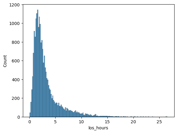
hm.get_los_stats(hills, by_category=False)
| count | mean | min | max | stdev | cv | skew | p50 | p75 | p95 | p99 | |
|---|---|---|---|---|---|---|---|---|---|---|---|
| all | 20247 | 3.1 | 0.1 | 26.6 | 2.6 | 0.8 | 2.3 | 2.2 | 3.6 | 8.7 | 12.9 |
plots - Daily and weekly summary plots#
hills['plots'].keys()
dict_keys(['ssu_summer24_occupancy_plot_week', 'ssu_summer24_arrivals_plot_week', 'ssu_summer24_departures_plot_week', 'ssu_summer24_occupancy_plot_Mon', 'ssu_summer24_occupancy_plot_Tue', 'ssu_summer24_occupancy_plot_Wed', 'ssu_summer24_occupancy_plot_Thu', 'ssu_summer24_occupancy_plot_Fri', 'ssu_summer24_occupancy_plot_Sat', 'ssu_summer24_occupancy_plot_Sun', 'ssu_summer24_arrivals_plot_Mon', 'ssu_summer24_arrivals_plot_Tue', 'ssu_summer24_arrivals_plot_Wed', 'ssu_summer24_arrivals_plot_Thu', 'ssu_summer24_arrivals_plot_Fri', 'ssu_summer24_arrivals_plot_Sat', 'ssu_summer24_arrivals_plot_Sun', 'ssu_summer24_departures_plot_Mon', 'ssu_summer24_departures_plot_Tue', 'ssu_summer24_departures_plot_Wed', 'ssu_summer24_departures_plot_Thu', 'ssu_summer24_departures_plot_Fri', 'ssu_summer24_departures_plot_Sat', 'ssu_summer24_departures_plot_Sun'])
hm.get_plot?
Signature:
hm.get_plot(
    hills: dict,
    flow_metric: str = 'occupancy',
    day_of_week: str = 'week',
)
Docstring:
Get plot object for specified flow metric and whether full week or specified day of week.

Parameters
----------
hills : dict
    Created by `make_hills`
flow_metric : str
    Either of 'arrivals', 'departures', 'occupancy' ('a', 'd', and 'o' are sufficient).
    Default='occupancy'
day_of_week : str
    Either of 'week', 'Sun', 'Mon', 'Tue', 'Wed', 'Thu', 'Fri', 'Sat'. Default='week'

Returns
-------
plot object from matplotlib
File:      ~/Documents/projects/hillmaker/src/hillmaker/hills.py
Type:      function
hm.get_plot(hills, 'o', day_of_week='Mon')

hm.get_plot(hills, 'o', 'week')
settings - Scenario settings#
hills['settings']
{'scenario_name': 'ssu_summer24',
 'in_field': 'InRoomTS',
 'out_field': 'OutRoomTS',
 'start_analysis_dt': numpy.datetime64('2024-06-01T00:00:00.000000000'),
 'end_analysis_dt': numpy.datetime64('2024-06-01T00:00:00.000000000'),
 'cat_field': 'PatType',
 'occ_weight_field': None,
 'bin_size_minutes': 30,
 'los_units': 'hours',
 'edge_bins': <EdgeBinsEnum.FRACTIONAL: 1>,
 'highres_bin_size_minutes': 30}
runtime - Total runtime in seconds#
hills['runtime']
21.24074344
Using a config file#
Instead of passing a bunch of arguments to make_hills, you can use a TOML formatted config file. Here’s what an example config file might look like:
[scenario_data]
scenario_name = "ss_example_1_config"
data = "./data/ssu_2024.csv"

[fields]
in_field = "InRoomTS"
out_field = "OutRoomTS"
# Just remove the following line if no category field
cat_field = "PatType"

[analysis_dates]
start_analysis_dt = 2024-01-02
end_analysis_dt = 2024-03-30

[settings]
bin_size_minutes = 60
verbosity = 1
csv_export_path = './output'
plot_export_path = './output'

# Add any additional arguments here
# Strings should be surrounded in double quotes
# Floats and ints are specified in the normal way as values
# Dates are specified as shown above

# For arguments that take lists, the entries look
# just like Python lists and following the other rules above

# cats_to_exclude = ["IVT", "OTH"]
# percentiles = [0.5, 0.8, 0.9]

# For arguments that take dictionaries, do this:
# main_title_properties = {loc = 'left', fontsize = 16}
# subtitle_properties = {loc = 'left', style = 'italic'}
# legend_properties = {loc = 'best', frameon = true, facecolor = 'w'}
The sections headings, [scenario_data], [fields], and [analysis_dates] aren’t actually necessary. You could actually put all input parameters within the [settings] section. Including the other headings is just an organizational aid.
Warning
You MUST include the [settings] section header.
hills_config = hm.make_hills(config='./input/ssu_example_1_config.toml')
2024-01-16 09:53:48,904 - hillmaker.hills - INFO - Starting scenario ss_example_1_config
2024-01-16 09:53:57,130 - hillmaker.summarize - INFO - Created nonstationary summaries - ['PatType']
2024-01-16 09:53:58,808 - hillmaker.summarize - INFO - Created nonstationary summaries - []
2024-01-16 09:53:58,859 - hillmaker.summarize - INFO - Created stationary summaries - ['PatType']
2024-01-16 09:53:58,879 - hillmaker.summarize - INFO - Created stationary summaries - []
2024-01-16 09:54:00,445 - hillmaker.hills - INFO - bydatetime and summaries by datetime created (seconds): 11.5415
2024-01-16 09:54:00,553 - hillmaker.hills - INFO - By datetime exported to csv in ./output (seconds): 0.1066
2024-01-16 09:54:00,630 - hillmaker.hills - INFO - Summaries exported to csv in ./output (seconds): 0.0765
2024-01-16 09:54:01,691 - hillmaker.plotting - INFO - Full week plots created (seconds): 1.0618
2024-01-16 09:54:03,908 - hillmaker.plotting - INFO - Individual day of week plots created (seconds): 2.2022
2024-01-16 09:54:03,909 - hillmaker.hills - INFO - Total time (seconds): 14.9937
hills_config['settings']
{'scenario_name': 'ss_example_1_config',
 'in_field': 'InRoomTS',
 'out_field': 'OutRoomTS',
 'start_analysis_dt': numpy.datetime64('2024-01-02T00:00:00.000000000'),
 'end_analysis_dt': numpy.datetime64('2024-01-02T00:00:00.000000000'),
 'cat_field': 'PatType',
 'occ_weight_field': None,
 'bin_size_minutes': 60,
 'los_units': 'hours',
 'edge_bins': <EdgeBinsEnum.FRACTIONAL: 1>,
 'highres_bin_size_minutes': 60}